
Audio Classification with Computer Vision
The ESC-50 dataset is a labeled collection of 2000 environmental audio recordings suitable for benchmarking methods of environmental sound classification.
The dataset consists of 5-second-long recordings organized into 50 semantical classes (with 40 examples per class) loosely arranged into 5 major categories:
import numpy as np
from matplotlib import pyplot as plt
from numpy.lib import stride_tricks
import os
import pandas as pd
import scipy.io.wavfile as wav
Visualize the Dataset
esc50_df = pd.read_csv('dataset/ESC-50/esc50.csv')
esc50_df.head()
| filename | fold | target | category | esc10 | src_file | take | |
|---|---|---|---|---|---|---|---|
| 0 | 1-100032-A-0.wav | 1 | 0 | dog | True | 100032 | A |
| 1 | 1-100038-A-14.wav | 1 | 14 | chirping_birds | False | 100038 | A |
| 2 | 1-100210-A-36.wav | 1 | 36 | vacuum_cleaner | False | 100210 | A |
| 3 | 1-100210-B-36.wav | 1 | 36 | vacuum_cleaner | False | 100210 | B |
| 4 | 1-101296-A-19.wav | 1 | 19 | thunderstorm | False | 101296 | A |
esc50_df['category'].value_counts()
dog 40 glass_breaking 40 drinking_sipping 40 rain 40 insects 40 laughing 40 hen 40 engine 40 breathing 40 crying_baby 40 hand_saw 40 coughing 40 snoring 40 chirping_birds 40 toilet_flush 40 pig 40 washing_machine 40 clock_tick 40 sneezing 40 rooster 40 sea_waves 40 siren 40 cat 40 door_wood_creaks 40 helicopter 40 crackling_fire 40 car_horn 40 brushing_teeth 40 vacuum_cleaner 40 thunderstorm 40 door_wood_knock 40 can_opening 40 crow 40 clapping 40 fireworks 40 chainsaw 40 airplane 40 mouse_click 40 pouring_water 40 train 40 sheep 40 water_drops 40 church_bells 40 clock_alarm 40 keyboard_typing 40 wind 40 footsteps 40 frog 40 cow 40 crickets 40 Name: category, dtype: int64
def fourier_transformation(sig, frameSize, overlapFac=0.5, window=np.hanning):
    win = window(frameSize)
    hopSize = int(frameSize - np.floor(overlapFac * frameSize))

    # zeros at beginning (thus center of 1st window should be for sample nr. 0)
    samples = np.append(np.zeros(int(np.floor(frameSize/2.0))), sig)
    # cols for windowing
    cols = np.ceil( (len(samples) - frameSize) / float(hopSize)) + 1
    # zeros at end (thus samples can be fully covered by frames)
    samples = np.append(samples, np.zeros(frameSize))

    frames = stride_tricks.as_strided(samples, shape=(int(cols), frameSize), strides=(samples.strides[0]*hopSize, samples.strides[0])).copy()
    frames *= win

    return np.fft.rfft(frames)
def make_logscale(spec, sr=44100, factor=20.):
    timebins, freqbins = np.shape(spec)

    scale = np.linspace(0, 1, freqbins) ** factor
    scale *= (freqbins-1)/max(scale)
    scale = np.unique(np.round(scale))

    # create spectrogram with new freq bins
    newspec = np.complex128(np.zeros([timebins, len(scale)]))
    for i in range(0, len(scale)):
        if i == len(scale)-1:
            newspec[:,i] = np.sum(spec[:,int(scale[i]):], axis=1)
        else:
            newspec[:,i] = np.sum(spec[:,int(scale[i]):int(scale[i+1])], axis=1)

    # list center freq of bins
    allfreqs = np.abs(np.fft.fftfreq(freqbins*2, 1./sr)[:freqbins+1])
    freqs = []
    for i in range(0, len(scale)):
        if i == len(scale)-1:
            freqs += [np.mean(allfreqs[int(scale[i]):])]
        else:
            freqs += [np.mean(allfreqs[int(scale[i]):int(scale[i+1])])]

    return newspec, freqs
def plot_spectrogram(location, categorie, plotpath=None, binsize=2**10, colormap="jet"):
    samplerate, samples = wav.read(location)

    s = fourier_transformation(samples, binsize)

    sshow, freq = make_logscale(s, factor=1.0, sr=samplerate)

    ims = 20.*np.log10(np.abs(sshow)/10e-6) # amplitude to decibel

    timebins, freqbins = np.shape(ims)

    print("timebins: ", timebins)
    print("freqbins: ", freqbins)

    plt.figure(figsize=(15, 7.5))
    plt.title('Class Label: ' + categorie)
    plt.imshow(np.transpose(ims), origin="lower", aspect="auto", cmap=colormap, interpolation="none")
    plt.colorbar()

    plt.xlabel("time (s)")
    plt.ylabel("frequency (hz)")
    plt.xlim([0, timebins-1])
    plt.ylim([0, freqbins])

    xlocs = np.float32(np.linspace(0, timebins-1, 5))
    plt.xticks(xlocs, ["%.02f" % l for l in ((xlocs*len(samples)/timebins)+(0.5*binsize))/samplerate])
    ylocs = np.int16(np.round(np.linspace(0, freqbins-1, 10)))
    plt.yticks(ylocs, ["%.02f" % freq[i] for i in ylocs])

    if plotpath:
        plt.savefig(plotpath, bbox_inches="tight")
    else:
        plt.show()

    plt.clf()

    return ims
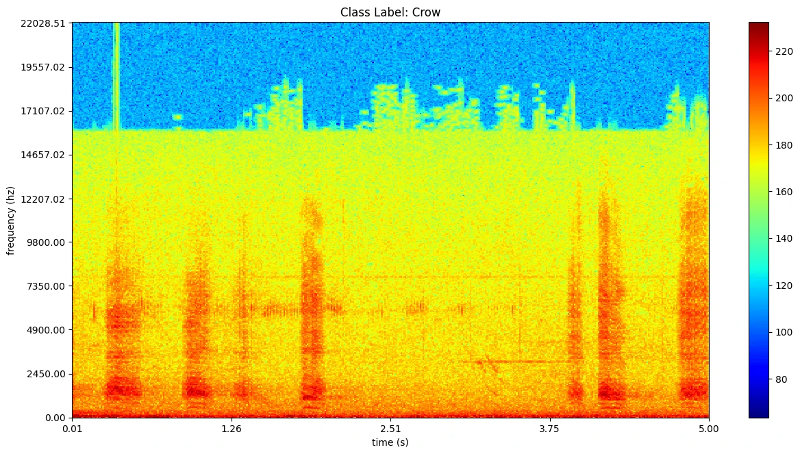
plot = plot_spectrogram('dataset/ESC-50/audio/' + esc50_df[esc50_df['category'] == 'crow']['filename'].iloc[0], categorie='Crow')
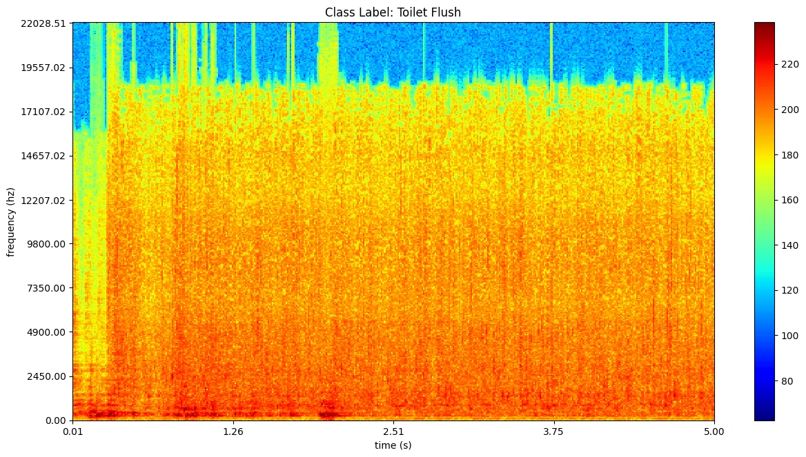
plot = plot_spectrogram('dataset/ESC-50/audio/' + esc50_df[esc50_df['category'] == 'toilet_flush']['filename'].iloc[0], categorie='Toilet Flush')
Data Preprocessing
def audio_vis(location, filepath, binsize=2**10, colormap="jet"):
    samplerate, samples = wav.read(location)

    s = fourier_transformation(samples, binsize)

    sshow, freq = make_logscale(s, factor=1.0, sr=samplerate)

    with np.errstate(divide='ignore'):
        ims = 20.*np.log10(np.abs(sshow)/10e-6) # amplitude to decibel

    timebins, freqbins = np.shape(ims)

    plt.figure(figsize=(15, 7.5))
    plt.imshow(np.transpose(ims), origin="lower", aspect="auto", cmap=colormap, interpolation="none")

    plt.axis('off')
    plt.xlim([0, timebins-1])
    plt.ylim([0, freqbins])

    plt.savefig(filepath, bbox_inches="tight")
    plt.close()

    return
conversion = []

for i in range(len(esc50_df.index)):

    filename = esc50_df['filename'].iloc[i]
    location = 'dataset/ESC-50/audio/' + filename
    category = esc50_df['category'].iloc[i]
    catpath = 'dataset/ESC-50/spectrogram/' + category
    filepath = catpath + '/' + filename[:-4] + '.jpg'

    conversion.append({location, filepath})
conversion[0]
for i in range(len(esc50_df.index)):

    filename = esc50_df['filename'].iloc[i]
    location = 'dataset/ESC-50/audio/' + filename
    category = esc50_df['category'].iloc[i]
    catpath = 'dataset/ESC-50/spectrogram/' + category
    filepath = catpath + '/' + filename[:-4] + '.jpg'

    os.makedirs(catpath, exist_ok=True)

    audio_vis(location, filepath)
Train-Test-Split
!pip install split-folders
import splitfolders
input_folder = 'dataset/ESC-50/spectrogram'
output = 'data'

splitfolders.ratio(input_folder, output=output, seed=42, ratio=(.8, .2))
Prepare Validation Data
testing = [
    'data/test/helicopter.wav',
    'data/test/cat.wav'
]
def test_vis(location, filepath, binsize=2**10, colormap="jet"):
    samplerate, samples = wav.read(location)

    s = fourier_transformation(samples, binsize)

    sshow, freq = make_logscale(s, factor=1.0, sr=samplerate)

    with np.errstate(divide='ignore'):
        ims = 20.*np.log10(np.abs(sshow)/10e-6) # amplitude to decibel

    timebins, freqbins = np.shape(ims)

    plt.figure(figsize=(15, 7.5))
    plt.imshow(np.transpose(ims), origin="lower", aspect="auto", cmap=colormap, interpolation="none")

    plt.axis('off')
    plt.xlim([0, timebins-1])
    plt.ylim([0, freqbins])

    plt.savefig(filepath, bbox_inches="tight")
    plt.close()

    return
test_vis(testing[0], filepath='data/test/helicopter.jpg')
test_vis(testing[1], filepath='data/test/cat.jpg')
Model Training
from ultralytics import YOLO
model = YOLO('yolov8n-cls.pt')
#model = YOLO('yolov8s-cls.pt')
results = model.train(data='./data', epochs=20, imgsz=640)
metrics = model.val()
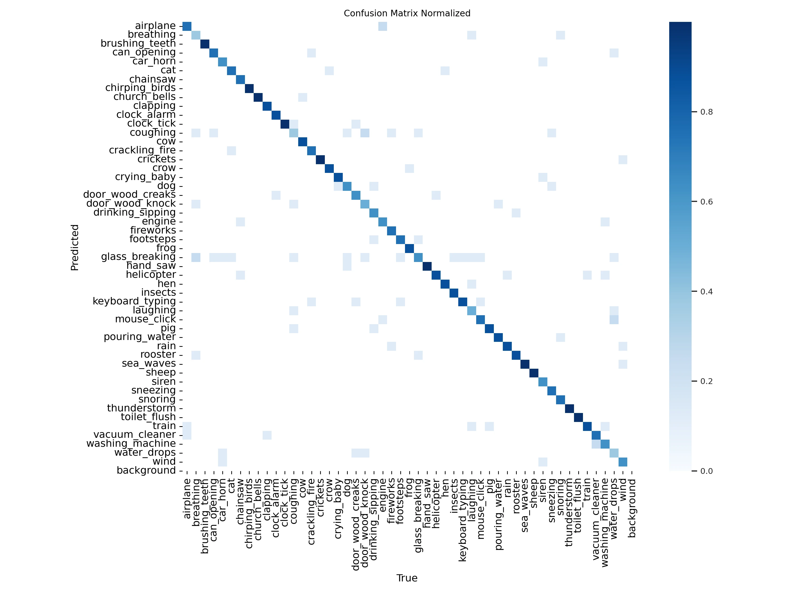
print(metrics.top1)
print(metrics.top5)
0.7824999690055847 0.9524999856948853
Model Predictions
# Predict with the model
pred = model('data/test/helicopter.jpg')

# helicopter 0.56, crying_baby 0.09, crickets 0.08, sea_waves 0.07, snoring 0.07, 3.5ms
# Speed: 4.9ms preprocess, 3.5ms inference, 0.1ms postprocess per image at shape (1, 3, 640, 640)
# Predict with the model
pred = model('data/test/cat.jpg')

# cat 0.55, rooster 0.23, crying_baby 0.22, laughing 0.00, siren 0.00, 3.5ms
# Speed: 13.0ms preprocess, 3.5ms inference, 0.1ms postprocess per image at shape (1, 3, 640, 640)