Sham Sui Po, Hong Kong

Analyzing Credit Card Customer Churn Behaviour

Analyzing Credit Card Customer Churn Behaviour

Problem Statement: A manager at the bank is disturbed with more and more customers leaving their credit card services. They would really appreciate if one could predict for them who is considering leaving the bank so they can proactively go to the customer to provide them better services and reverse the customers' decision in their favour.

Github Repository

Analyzing Credit Card Customer Churn Behaviour

Dataset


Clientnum	Num Client number. Unique identifier for the customer holding the account
Attrition_Flag	char Internal event (customer activity) variable
Customer_Age	Num Demographic variable - Customer's Age in Years
Gender	Char Demographic variable - M=Male, F=Female
Dependent_count	Num Demographic variable - Number of people dependents
Education_Level	Char Demographic variable - Educational Qualification of the account holder(example: high school, college graduate, etc.)
Marital_Status	Char Demographic variable - Married, Single, Unknown
Income_Category	Char Demographic variable - Annual Income Category of the account holder (< 40K, 40K - 60K, 60K - 80K, 80K-120K, > 120K, Unknown)
Card_Category	Char Product Variable - Type of Card (Blue, Silver, Gold, Platinum)
Months_on_book	Num Months on book (Time of Relationship)
Total_Relationship_Count	Num Total no. of products held by the customer
Months_Inactive_12_mon	Num No. of months inactive in the last 12 months
Contacts_Count_12_mon	Num No. of Contacts in the last 12 months
Credit_Limit	Num Credit Limit on the Credit Card
Total_Revolving_Bal	Num Total Revolving Balance on the Credit Card
Avg_Open_To_Buy	Num Open to Buy Credit Line (Average of last 12 months)
Total_Amt_Chng_Q4_Q1	Num Change in Transaction Amount (Q4 over Q1)
Total_Trans_Amt	Num Total Transaction Amount (Last 12 months)
Total_Trans_Ct	Num Total Transaction Count (Last 12 months)
Total_Ct_Chng_Q4_Q1	Num Change in Transaction Count (Q4 over Q1)
Avg_Utilization_Ratio	Num Average Card Utilization Ratio

!wget https://github.com/tassneam/Credit-Card-Customers-Prediction/raw/main/BankChurners.csv -P dataset

import matplotlib.pyplot as plt
import numpy as np
import pandas as pd
import plotly.graph_objs as go
from plotly.offline import iplot
import seaborn as sns

cc_df = pd.read_csv('dataset/BankChurners.csv')
cc_df.head(5).transpose()
# 5 rows × 23 columns

	0	1	2	3	4
CLIENTNUM	768805383	818770008	713982108	769911858	709106358
Attrition_Flag	Existing Customer	Existing Customer	Existing Customer	Existing Customer	Existing Customer
Customer_Age	45	49	51	40	40
Gender	M	F	M	F	M
Dependent_count	3	5	3	4	3
Education_Level	High School	Graduate	Graduate	High School	Uneducated
Marital_Status	Married	Single	Married	Unknown	Married
Income_Category	60𝐾−80K	Less than 40K	80𝐾−120K	Less than 40K	60𝐾−80K
Card_Category	Blue	Blue	Blue	Blue	Blue
Months_on_book	39	44	36	34	21
Total_Relationship_Count	5	6	4	3	5
Months_Inactive_12_mon	1	1	1	4
Contacts_Count_12_mon	3	2	0	1	0
Credit_Limit	12691.0	8256.0	3418.0	3313.0	4716.0
Total_Revolving_Bal	777	864	0	2517	0
Avg_Open_To_Buy	11914.0	7392.0	3418.0	796.0	4716.0
Total_Amt_Chng_Q4_Q1	1.335	1.541	2.594	1.405	2.175
Total_Trans_Amt	1144	1291	1887	1171	816
Total_Trans_Ct	42	33	20	20	28
Total_Ct_Chng_Q4_Q1	1.625	3.714	2.333	2.333	2.5
Avg_Utilization_Ratio	0.061	0.105	0.0	0.76	0.0
Naive_Bayes_Classifier	0.000093	0.000057	0.000021	0.000134	0.000022
classification	True	True	True	True	True

Preprocessing

Duplicates

print(cc_df.shape, cc_df['CLIENTNUM'].nunique())
# there are as many ClientIDs as there are rows :thumbsup:
# (2998, 23) 2998

cc_df.drop_duplicates(inplace=True)
cc_df.shape
# nothing is dropped :thumbsup:
# (2998, 23)

Subsetting

cc_df.columns
# Index(['CLIENTNUM', 'Attrition_Flag', 'Customer_Age', 'Gender',
#        'Dependent_count', 'Education_Level', 'Marital_Status',
#        'Income_Category', 'Card_Category', 'Months_on_book',
#        'Total_Relationship_Count', 'Months_Inactive_12_mon',
#        'Contacts_Count_12_mon', 'Credit_Limit', 'Total_Revolving_Bal',
#        'Avg_Open_To_Buy', 'Total_Amt_Chng_Q4_Q1', 'Total_Trans_Amt',
#        'Total_Trans_Ct', 'Total_Ct_Chng_Q4_Q1', 'Avg_Utilization_Ratio',
#        'Naive_Bayes_Classifier', 'classification'],
#       dtype='object')

# drop what you don't need
cc_df_ss = cc_df[['CLIENTNUM', 'Attrition_Flag', 'Customer_Age', 'Gender',
       'Dependent_count', 'Education_Level', 'Marital_Status',
       'Income_Category', 'Card_Category', 'Months_on_book',
       'Total_Relationship_Count', 'Months_Inactive_12_mon',
       'Contacts_Count_12_mon', 'Credit_Limit', 'Total_Revolving_Bal',
       'Avg_Open_To_Buy', 'Total_Amt_Chng_Q4_Q1', 'Total_Trans_Amt',
       'Total_Trans_Ct', 'Total_Ct_Chng_Q4_Q1', 'Avg_Utilization_Ratio']]

cc_df_ss.shape
# (2998, 21)

Datatypes

# check if int/float/datetime values are not strings
cc_df_ss.dtypes


CLIENTNUM	int64
Attrition_Flag	object
Customer_Age	int64
Gender	object
Dependent_count	int64
Education_Level	object
Marital_Status	object
Income_Category	object
Card_Category	object
Months_on_book	int64
Total_Relationship_Count	int64
Months_Inactive_12_mon	int64
Contacts_Count_12_mon	int64
Credit_Limit	float64
Total_Revolving_Bal	int64
Avg_Open_To_Buy	float64
Total_Amt_Chng_Q4_Q1	float64
Total_Trans_Amt	int64
Total_Trans_Ct	int64
Total_Ct_Chng_Q4_Q1	float64
Avg_Utilization_Ratio	float64
dtype: object

Missing Values

# test for missing data
cc_df_ss.isnull().sum()


CLIENTNUM	0
Attrition_Flag	0
Customer_Age	0
Gender	0
Dependent_count	0
Education_Level	0
Marital_Status	0
Income_Category	0
Card_Category	0
Months_on_book	0
Total_Relationship_Count	0
Months_Inactive_12_mon	0
Contacts_Count_12_mon	0
Credit_Limit	0
Total_Revolving_Bal	0
Avg_Open_To_Buy	0
Total_Amt_Chng_Q4_Q1	0
Total_Trans_Amt	0
Total_Trans_Ct	0
Total_Ct_Chng_Q4_Q1	0
Avg_Utilization_Ratio	0

Data Transformation

Binning

print(
    cc_df_ss['Customer_Age'].min(),
    cc_df_ss['Customer_Age'].max()
)
# 26 73 => bins=[20,30,40,50,60,70,80]

bins=[20,30,40,50,60,70,80]
labels=['20s','30s','40s','50s','60s','70s','80s']

cc_df_ss['Customer_Age_Bins'] = pd.cut(
    cc_df_ss['Customer_Age'],
    bins,
    labels,
    include_lowest=True
)

cc_df_ss.head(5).transpose()

	0	1	2	3	4
CLIENTNUM	768805383	818770008	713982108	769911858	709106358
Attrition_Flag	Existing Customer	Existing Customer	Existing Customer	Existing Customer	Existing Customer
Customer_Age	45	49	51	40	40
Gender	M	F	M	F	M
Dependent_count	3	5	3	4	3
Education_Level	High School	Graduate	Graduate	High School	Uneducated
Marital_Status	Married	Single	Married	Unknown	Married
Income_Category	60𝐾−80K	Less than 40K	80𝐾−120K	Less than 40K	60𝐾−80K
Card_Category	Blue	Blue	Blue	Blue	Blue
Months_on_book	39	44	36	34	21
Total_Relationship_Count	5	6	4	3	5
Months_Inactive_12_mon	1	1	1	4	1
Contacts_Count_12_mon	3	2	0	1	0
Credit_Limit	12691.0	8256.0	3418.0	3313.0	4716.0
Total_Revolving_Bal	777	864	0	2517	0
Avg_Open_To_Buy	11914.0	7392.0	3418.0	796.0	4716.0
Total_Amt_Chng_Q4_Q1	1.335	1.541	2.594	1.405	2.175
Total_Trans_Amt	1144	1291	1887	1171	816
Total_Trans_Ct	42	33	20	20	28
Total_Ct_Chng_Q4_Q1	1.625	3.714	2.333	2.333	2.5
Avg_Utilization_Ratio	0.061	0.105	0.0	0.76	0.0
Customer_Age_Bins	(40.0, 50.0]	(40.0, 50.0]	(50.0, 60.0]	(30.0, 40.0]	(30.0, 40.0]

Data Exploration

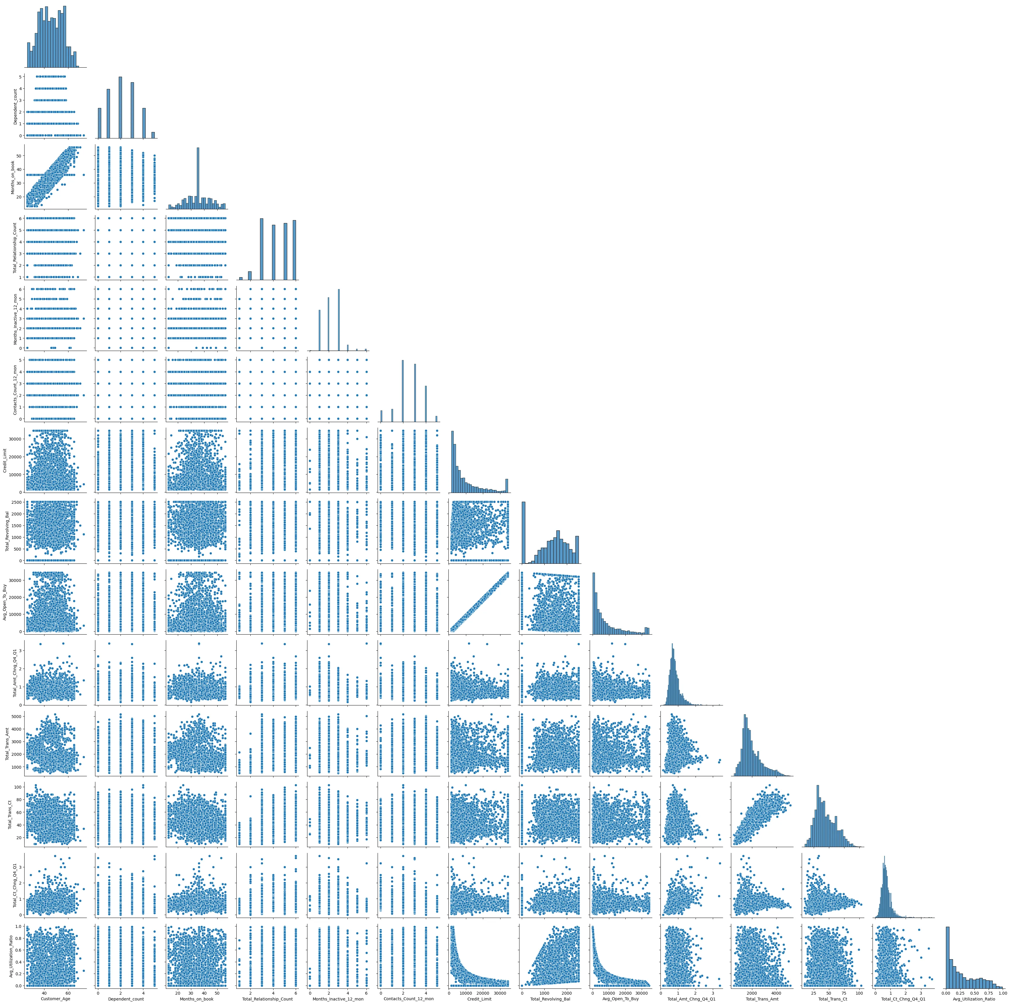
Scatterplots

cc_df_ss.columns

# find correlations using a pairplot
# remove unecessary columns
temp = cc_df_ss[['Attrition_Flag', 'Customer_Age', 'Gender',
       'Dependent_count', 'Education_Level', 'Marital_Status',
       'Income_Category', 'Card_Category', 'Months_on_book',
       'Total_Relationship_Count', 'Months_Inactive_12_mon',
       'Contacts_Count_12_mon', 'Credit_Limit', 'Total_Revolving_Bal',
       'Avg_Open_To_Buy', 'Total_Amt_Chng_Q4_Q1', 'Total_Trans_Amt',
       'Total_Trans_Ct', 'Total_Ct_Chng_Q4_Q1', 'Avg_Utilization_Ratio']]
# remove categorical columns
numeric_data_df = temp._get_numeric_data()
numeric_data_df.head(5).transpose()

	0	1	2	3	4
Customer_Age	45.000	49.000	51.000	40.000	40.000
Dependent_count	3.000	5.000	3.000	4.000	3.000
Months_on_book	39.000	44.000	36.000	34.000	21.000
Total_Relationship_Count	5.000	6.000	4.000	3.000	5.000
Months_Inactive_12_mon	1.000	1.000	1.000	4.000	1.000
Contacts_Count_12_mon	3.000	2.000	0.000	1.000	0.000
Credit_Limit	12691.000	8256.000	3418.000	3313.000	4716.000
Total_Revolving_Bal	777.000	864.000	0.000	2517.000	0.000
Avg_Open_To_Buy	11914.000	7392.000	3418.000	796.000	4716.000
Total_Amt_Chng_Q4_Q1	1.335	1.541	2.594	1.405	2.175
Total_Trans_Amt	1144.000	1291.000	1887.000	1171.000	816.000
Total_Trans_Ct	42.000	33.000	20.000	20.000	28.000
Total_Ct_Chng_Q4_Q1	1.625	3.714	2.333	2.333	2.500
Avg_Utilization_Ratio	0.061	0.105	0.000	0.760	0.000

pairgrid = sns.PairGrid(
    data=numeric_data_df,
    diag_sharey=False,
    corner=True
)

pairgrid.map_lower(sns.scatterplot)
pairgrid.map_diag(sns.histplot)

plt.savefig('../assets/CC_Customer_Churn_13.webp', bbox_inches='tight')

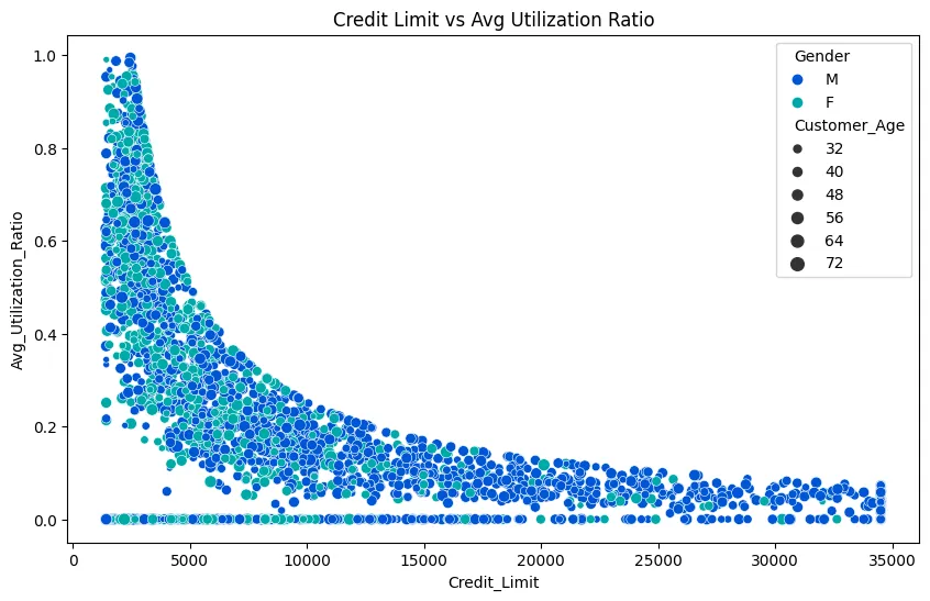
Credit Card Customer Churn Prediction

# dive deeper into plots with interesting correlations
plt.figure(figsize=(10, 6))

# hue/size by continuous column
sns.scatterplot(
    data=cc_df_ss,
    x='Credit_Limit',
    y='Avg_Utilization_Ratio',
    hue='Gender',
    palette='winter',
    size='Customer_Age'
).set_title('Credit Limit vs Avg Utilization Ratio')

plt.savefig('../assets/CC_Customer_Churn_14.webp', bbox_inches='tight')

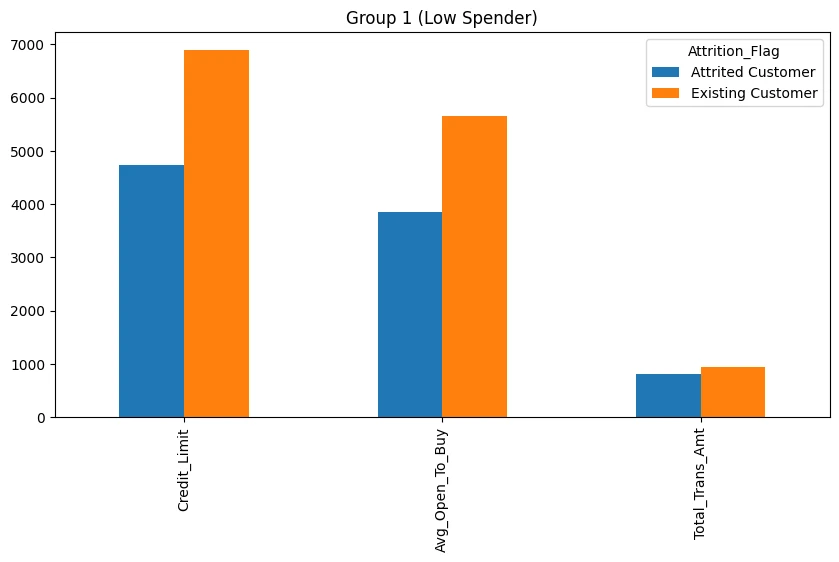
Credit Card Customer Churn Prediction

Investigate Subgroups

# compare high to low spender
bins = [
    cc_df_ss['Total_Trans_Amt'].min(),
    1000,
    cc_df_ss['Total_Trans_Amt'].max()
]

labels = ['Group 1', "Group 2"]

cc_df_ss_temp = cc_df_ss.copy()

cc_df_ss_temp['Total_Trans_Amt_Grp'] = pd.cut(
    cc_df_ss['Total_Trans_Amt'],
    bins=bins,
    labels=labels,
    include_lowest=True
)

cc_df_ss_temp.head(1).transpose()

	0
CLIENTNUM	768805383
Attrition_Flag	Existing Customer
Customer_Age	45
Gender	M
Dependent_count	3
Education_Level	High School
Marital_Status	Married
Income_Category	60𝐾−80K
Card_Category	Blue
Months_on_book	39
Total_Relationship_Count	5
Months_Inactive_12_mon	1
Contacts_Count_12_mon	3
Credit_Limit	12691.0
Total_Revolving_Bal	777
Avg_Open_To_Buy	11914.0
Total_Amt_Chng_Q4_Q1	1.335
Total_Trans_Amt	1144
Total_Trans_Ct	42
Total_Ct_Chng_Q4_Q1	1.625
Avg_Utilization_Ratio	0.061
Customer_Age_Bins	(40.0, 50.0]
Total_Trans_Amt_Grp	Group 2

cc_df_ss_temp = cc_df_ss_temp.groupby(['Total_Trans_Amt_Grp', 'Attrition_Flag']).agg({
    'CLIENTNUM':'nunique',
    'Customer_Age':'median',
    'Dependent_count':'median',
    'Months_on_book':'median',
    'Total_Relationship_Count':'median',
    'Months_Inactive_12_mon':'median',
    'Contacts_Count_12_mon':'median',
    'Credit_Limit':'median',
    'Total_Revolving_Bal':'median',
    'Avg_Open_To_Buy':'median',
    'Total_Amt_Chng_Q4_Q1':'median',
    'Total_Trans_Amt':'median',
    'Total_Trans_Ct':'median',
    'Total_Ct_Chng_Q4_Q1':'median',
    'Avg_Utilization_Ratio':'median',
})

cc_df_ss_temp.transpose()

Total_Trans_Amt_Grp	Group 1		Group 2
Attrition_Flag	Attrited Customer	Existing Customer	Attrited Customer	Existing Customer
CLIENTNUM	142.0000	19.000	82.00	2755.000
Customer_Age	49.0000	44.000	48.00	46.000
Dependent_count	2.0000	2.000	2.00	2.000
Months_on_book	36.0000	36.000	36.00	36.000
Total_Relationship_Count	3.0000	5.000	3.00	5.000
Months_Inactive_12_mon	3.0000	2.000	3.00	2.000
Contacts_Count_12_mon	3.0000	2.000	3.00	3.000
Credit_Limit	4740.5000	6884.000	7618.00	5550.000
Total_Revolving_Bal	0.0000	1330.000	0.00	1475.000
Avg_Open_To_Buy	3854.0000	5653.000	6410.00	4237.000
Total_Amt_Chng_Q4_Q1	0.7250	0.781	0.77	0.761
Total_Trans_Amt	810.0000	949.000	1353.00	1805.000
Total_Trans_Ct	20.0000	24.000	33.00	43.000
Total_Ct_Chng_Q4_Q1	0.4645	0.909	0.46	0.682
Avg_Utilization_Ratio	0.0000	0.152	0.00	0.210

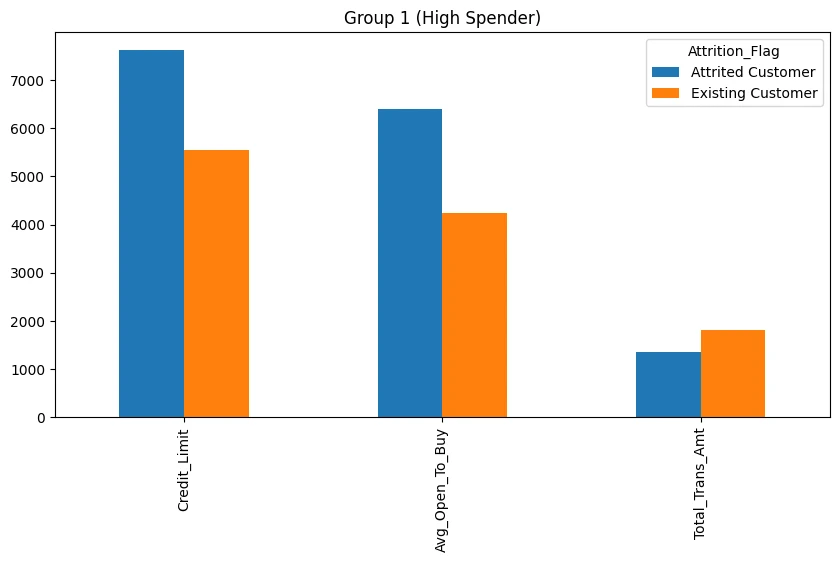
cc_df_ss_temp.transpose()['Group 1'].loc[
    [
        'Credit_Limit',
        'Avg_Open_To_Buy',
        'Total_Trans_Amt'
    ]
]

Attrition_Flag	Attrited Customer	Existing Customer
Credit_Limit	4740.5	6884.0
Avg_Open_To_Buy	3854.0	5653.0
Total_Trans_Amt	810.0	949.0

cc_df_ss_temp.transpose()['Group 1'].loc[
    ['Credit_Limit','Avg_Open_To_Buy','Total_Trans_Amt']
].plot.bar(
    figsize=(10,5),
    subplots=False,
    legend=True,
    sharey=True,
    layout=(1,2),
    title='Group 1 (Low Spender)'
)

Credit Card Customer Churn Prediction

cc_df_ss_temp.transpose()['Group 2'].loc[
    ['Credit_Limit','Avg_Open_To_Buy','Total_Trans_Amt']
].plot.bar(
    figsize=(10,5),
    subplots=False,
    legend=True,
    sharey=True,
    layout=(1,2),
    title='Group 1 (High Spender)'
)

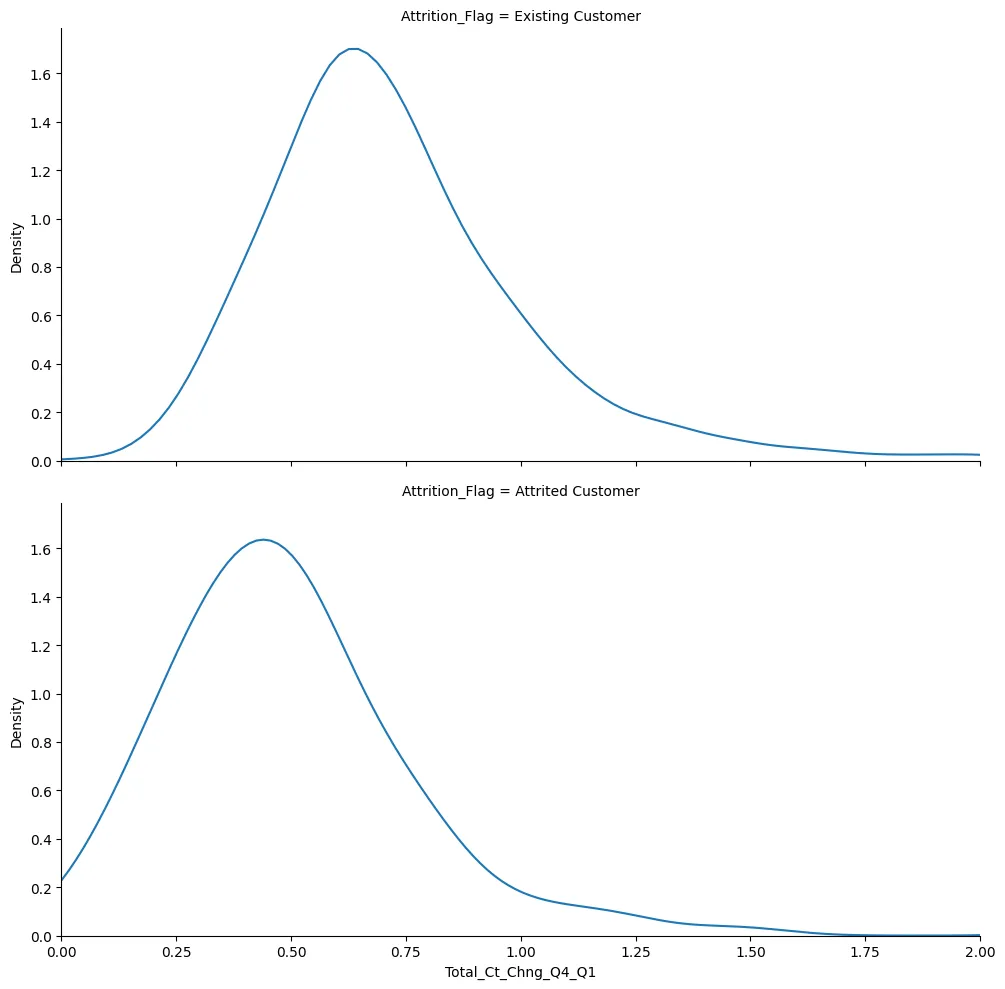
Credit Card Customer Churn Prediction

plot = sns.FacetGrid(
    cc_df_ss,
    row='Attrition_Flag',
    height=5,
    aspect=2
)

plot.map_dataframe(
    sns.kdeplot,
    x='Total_Ct_Chng_Q4_Q1'
)

plt.xlim(0,2)

plt.savefig('../assets/CC_Customer_Churn_15.webp', bbox_inches='tight')

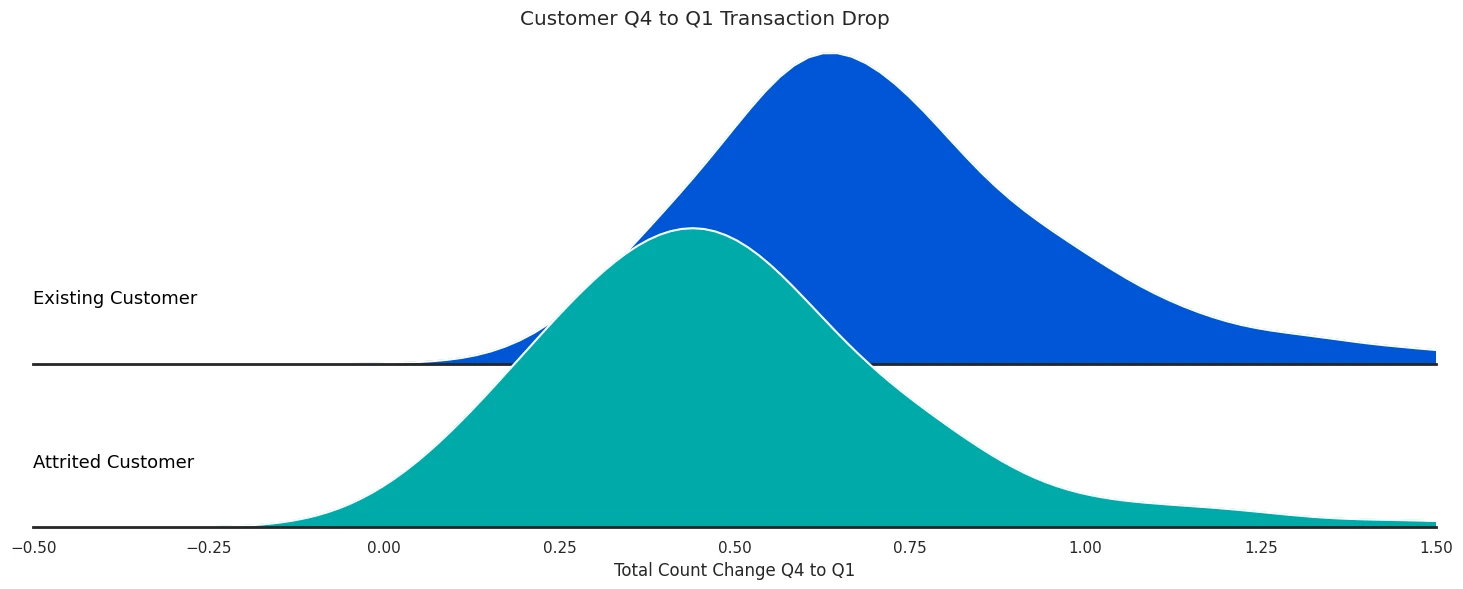
Credit Card Customer Churn Prediction

palette = sns.color_palette('winter', 2)

def label(x, color, label):
    ax = plt.gca()
    ax.text(0, .2, label, color='black', fontsize=13,
           ha='left', va='center', transform=ax.transAxes)

sns.set_theme(
    style='white',
    rc={'axes.facecolor': (0, 0, 0, 0), 'axes.linewidth':2}
)

fg = sns.FacetGrid(
    cc_df_ss,
    palette=palette,
    hue='Attrition_Flag',
    row='Attrition_Flag',
    aspect=5,
    height=3
)

fg.map_dataframe(
    sns.kdeplot,
    x='Total_Ct_Chng_Q4_Q1',
    fill=True,
    alpha=1
)

fg.map_dataframe(
    sns.kdeplot,
    x='Total_Ct_Chng_Q4_Q1',
    color='white'
)

fg.map(label, 'Attrition_Flag')
fg.fig.subplots_adjust(hspace=-.5)
fg.set_titles('')
fg.set(yticks=[], ylabel='', xlabel='Total Count Change Q4 to Q1')
fg.despine(left=True)

plt.suptitle('Customer Q4 to Q1 Transaction Drop', y=0.98)
plt.xlim(-0.5,1.5)

Credit Card Customer Churn Prediction

Histograms

plt.hist( 
    cc_df_ss['Customer_Age'],
    bins=7,
    histtype='step'
)
plt.title('Customer Age Histogram')
plt.xlabel('Age Group')
plt.ylabel('Count')

Credit Card Customer Churn Prediction

# find churn percentage
cc_df_ss['Attrition_Flag'].value_counts()

# Existing Customer    2774
# Attrited Customer     224
# Name: Attrition_Flag, dtype: int64

percentage = cc_df_ss['Attrition_Flag'].value_counts()['Attrited Customer'] / cc_df_ss.shape[0] * 100
print(f"Attrited Customers: {round(percentage)}%")

# Attrited Customers: 7%

plt.hist(
    cc_df_ss['Months_on_book'],
    bins=20,
    histtype='step'
)

plt.title('Customer Months on book (Time of Relationship)')
plt.xlabel('Months on Book')
plt.ylabel('Count')

Credit Card Customer Churn Prediction

plt.hist(
    cc_df_ss['Credit_Limit'],
)

plt.vlines(
    x=cc_df_ss['Credit_Limit'].mean(),
    ymin=0, ymax=1500, colors='0.75',
    linestyles='dashed', label='MEAN'
)

plt.vlines(
    x=cc_df_ss['Credit_Limit'].median(),
    ymin=0, ymax=1500, colors='0.75',
    linestyles='dotted', label='MEDIAN'
)

plt.title('Customer Credit Limit on the Credit Card')
plt.xlabel('Credit Limit')
plt.ylabel('Count')
plt.legend()

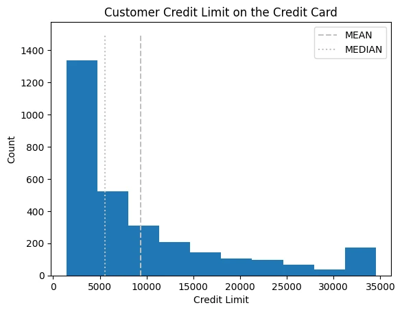
Credit Card Customer Churn Prediction

The Mean is more influenced by outliers than the Median function. Use median() when your distribution deviates from a normal distribution.

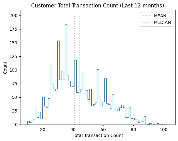
plt.hist(
    cc_df_ss['Total_Trans_Ct'],
    bins=75,
    histtype='step'
)

plt.vlines(
    x=cc_df_ss['Total_Trans_Ct'].mean(),
    ymin=0, ymax=200, colors='0.75',
    linestyles='dashed', label='MEAN'
)

plt.vlines(
    x=cc_df_ss['Total_Trans_Ct'].median(),
    ymin=0, ymax=200, colors='0.75',
    linestyles='dotted', label='MEDIAN'
)

plt.title('Customer Total Transaction Count (Last 12 months)')
plt.xlabel('Total Transaction Count')
plt.ylabel('Count')
plt.legend()

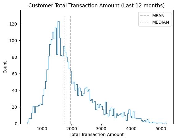
Credit Card Customer Churn Prediction

plt.hist(
    cc_df_ss['Total_Trans_Amt'],
    bins=100,
    histtype='step'
)

plt.vlines(
    x=cc_df_ss['Total_Trans_Amt'].mean(),
    ymin=0, ymax=130, colors='0.75',
    linestyles='dashed', label='MEAN'
)

plt.vlines(
    x=cc_df_ss['Total_Trans_Amt'].median(),
    ymin=0, ymax=130, colors='0.75',
    linestyles='dotted', label='MEDIAN'
)

plt.title('Customer Total Transaction Amount (Last 12 months)')
plt.xlabel('Total Transaction Amount')
plt.ylabel('Count')
plt.legend()

Credit Card Customer Churn Prediction

Data Transformation

Normalization

def normalize(column):
    upper = column.max()
    lower = column.min()
    norm = (column - lower)/(upper - lower)
    
    return norm

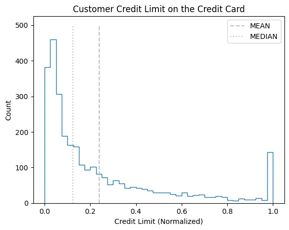
cc_df_ss['Credit_Limit_Norm'] = normalize(cc_df_ss['Credit_Limit'])

plt.hist(
    x=cc_df_ss['Credit_Limit_Norm'],
    bins=40,
    histtype='step'
)

plt.vlines(
    x=cc_df_ss['Credit_Limit_Norm'].mean(),
    ymin=0, ymax=500, colors='0.75',
    linestyles='dashed', label='MEAN'
)

plt.vlines(
    x=cc_df_ss['Credit_Limit_Norm'].median(),
    ymin=0, ymax=500, colors='0.75',
    linestyles='dotted', label='MEDIAN'
)

plt.title('Customer Credit Limit on the Credit Card')
plt.xlabel('Credit Limit (Normalized)')
plt.ylabel('Count')
plt.legend()

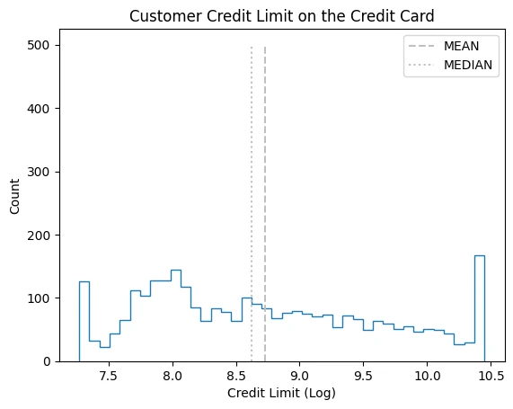
Credit Card Customer Churn Prediction

Log Transform

cc_df_ss['Credit_Limit_Log'] = np.log(cc_df_ss['Credit_Limit'])

plt.hist(
    x=cc_df_ss['Credit_Limit_Log'],
    bins=40,
    histtype='step'
)

plt.vlines(
    x=cc_df_ss['Credit_Limit_Log'].mean(),
    ymin=0, ymax=500, colors='0.75',
    linestyles='dashed', label='MEAN'
)

plt.vlines(
    x=cc_df_ss['Credit_Limit_Log'].median(),
    ymin=0, ymax=500, colors='0.75',
    linestyles='dotted', label='MEDIAN'
)

plt.title('Customer Credit Limit on the Credit Card')
plt.xlabel('Credit Limit (Log)')
plt.ylabel('Count')
plt.legend()

Credit Card Customer Churn Prediction

fig, axes = plt.subplots(1, 3, figsize=(15, 5))
fig.suptitle('Before and After Transformation')

sns.histplot(
    data=cc_df_ss,
    x='Credit_Limit',
    bins=50,
    hue='Gender',
    palette='winter',
    kde=True,
    ax=axes[0]
)

sns.histplot(
    data=cc_df_ss,
    x='Credit_Limit_Norm',
    bins=50,
    hue='Gender',
    palette='winter',
    kde=True,
    ax=axes[1]
)

sns.histplot(
    data=cc_df_ss,
    x='Credit_Limit_Log',
    bins=50,
    hue='Gender',
    palette='winter',
    kde=True,
    ax=axes[2]
)

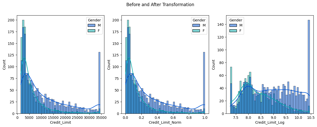
Credit Card Customer Churn Prediction

More Distribution Plot

Box Plot

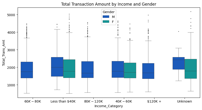
plt.figure(figsize=(10, 5))
plt.title('Total Transaction Amount by Income and Gender')
  
plot = sns.boxplot(
    data=cc_df_ss,
    y='Total_Trans_Amt',
    x='Income_Category',
    hue='Gender',
    palette='winter',
    orient='v',
    linewidth=0.5,
    fliersize=1
)

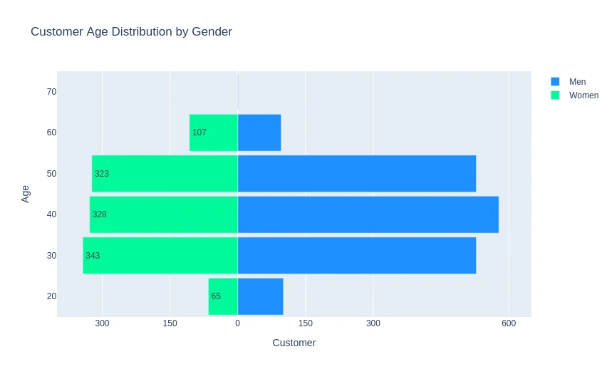
Credit Card Customer Churn Prediction

Pyramid Chart

# count customers in age bins and classify by gender
cc_gen_age = cc_df_ss.groupby(
    ['Gender', 'Customer_Age_Bins']
)['CLIENTNUM'].nunique().reset_index()

cc_gen_age.head(5)

	Gender	Customer_Age_Bins	CLIENTNUM
0	F	(19.999, 30.0]	65
1	F	(30.0, 40.0]	343
2	F	(40.0, 50.0]	328
3	F	(50.0, 60.0]	323
4	F	(60.0, 70.0]	107

women_bins = np.array(-1 * cc_gen_age[cc_gen_age['Gender'] == 'F']['CLIENTNUM'])
men_bins = np.array(cc_gen_age[cc_gen_age['Gender'] == 'M']['CLIENTNUM'])
y = list(range(20, 100, 10))

layout = go.Layout(
      title='Customer Age Distribution by Gender',
       yaxis=go.layout.YAxis(title='Age'),
       xaxis=go.layout.XAxis(
           range=[-400, 650],
           tickvals=[-300, -150, 0, 150, 300, 600],
           ticktext=[300, 150, 0, 150, 300, 600],
           title='Customer'),
       barmode='overlay',
       bargap=0.1)

p_data = [go.Bar(y=y,
               x=men_bins,
               orientation='h',
               name='Men',
               hoverinfo='x',
               marker=dict(color='dodgerblue')
               ),
        go.Bar(y=y,
               x=woman_bins,
               orientation='h',
               name='Women',
               text=-1 * women_bins.astype('int'),
               hoverinfo='text',
               marker=dict(color='mediumspringgreen')
               )]

iplot(dict(data=p_data, layout=layout))

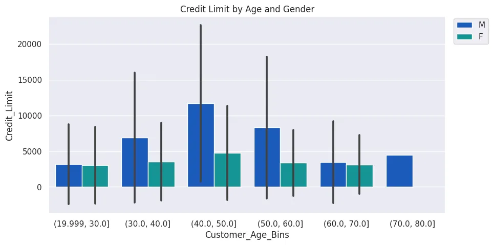
Credit Card Customer Churn Prediction

Bar Chart

plt.figure(figsize=(10, 5))
plt.title('Credit Limit by Age and Gender')
sns.set(style='darkgrid')
sns.barplot(
    data=cc_df_ss,
    x='Customer_Age_Bins',
    y='Credit_Limit',
    estimator=np.median,
    errorbar='sd',
    hue='Gender',
    palette='winter'
)
plt.legend(bbox_to_anchor=(1.01,1.01))
plt.savefig('../assets/CC_Customer_Churn_11.webp', bbox_inches='tight')

Credit Card Customer Churn Prediction

Aggregations

cc_df_attr = cc_df_ss.groupby(['Attrition_Flag']).agg({
    'CLIENTNUM':'nunique',
    'Customer_Age':'median',
    'Dependent_count':'median',
    'Months_on_book':'median',
    'Total_Relationship_Count':'median',
    'Months_Inactive_12_mon':'median',
    'Contacts_Count_12_mon':'median',
    'Credit_Limit':'median',
    'Total_Revolving_Bal':'median',
    'Avg_Open_To_Buy':'median',
    'Total_Amt_Chng_Q4_Q1':'median',
    'Total_Trans_Amt':'median',
    'Total_Trans_Ct':'median',
    'Total_Ct_Chng_Q4_Q1':'median',
    'Avg_Utilization_Ratio':'median',
})

cc_df_attr_trans = cc_df_attr.transpose().reset_index()
cc_df_attr_trans

Attrition_Flag	index	Attrited Customer	Existing Customer
0	CLIENTNUM	224.0000	2774.000
1	Customer_Age	48.0000	46.000
2	Dependent_count	2.0000	2.000
3	Months_on_book	36.0000	36.000
4	Total_Relationship_Count	3.0000	5.000
5	Months_Inactive_12_mon	3.0000	2.000
6	Contacts_Count_12_mon	3.0000	3.000
7	Credit_Limit	5687.5000	5553.000
8	Total_Revolving_Bal	0.0000	1474.500
9	Avg_Open_To_Buy	5189.5000	4245.000
10	Total_Amt_Chng_Q4_Q1	0.7375	0.762
11	Total_Trans_Amt	911.0000	1802.000
12	Total_Trans_Ct	24.0000	42.000
13	Total_Ct_Chng_Q4_Q1	0.4620	0.682
14	Avg_Utilization_Ratio	0.0000	0.209

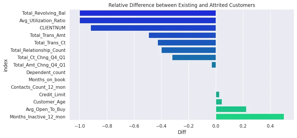
# sort by greatest difference
cc_df_attr_trans['Diff'] = cc_df_attr_trans['Attrited Customer'] / cc_df_attr_trans['Existing Customer'] - 1
cc_df_attr_trans = cc_df_attr_trans.sort_values('Diff')
cc_df_attr_trans

Attrition_Flag	index	Attrited Customer	Existing Customer	Diff
8	Total_Revolving_Bal	0.0000	1474.500	-1.000000
14	Avg_Utilization_Ratio	0.0000	0.209	-1.000000
0	CLIENTNUM	224.0000	2774.000	-0.919250
11	Total_Trans_Amt	911.0000	1802.000	-0.494451
12	Total_Trans_Ct	24.0000	42.000	-0.428571
4	Total_Relationship_Count	3.0000	5.000	-0.400000
13	Total_Ct_Chng_Q4_Q1	0.4620	0.682	-0.322581
10	Total_Amt_Chng_Q4_Q1	0.7375	0.762	-0.032152
2	Dependent_count	2.0000	2.000	0.000000
3	Months_on_book	36.0000	36.000	0.000000
6	Contacts_Count_12_mon	3.0000	3.000	0.000000
7	Credit_Limit	5687.5000	5553.000	0.024221
1	Customer_Age	48.0000	46.000	0.043478
9	Avg_Open_To_Buy	5189.5000	4245.000	0.222497
5	Months_Inactive_12_mon	3.0000	2.000	0.500000

plt.figure(figsize=(10, 5))
plt.title('Relative Difference between Existing and Attrited Customers')
sns.set(style='darkgrid')
sns.barplot(
    data=cc_df_attr_trans,
    x='Diff',
    y='index',
    estimator=np.median,
    errorbar='sd',
    palette='winter',
    orient='h'
)

plt.savefig('../assets/CC_Customer_Churn_12.webp', bbox_inches='tight')

Credit Card Customer Churn Prediction

Analyzing Credit Card Customer Churn Behaviour

Dataset​

Preprocessing​

Duplicates​

Subsetting​

Datatypes​

Missing Values​

Data Transformation​

Binning​

Data Exploration​

Scatterplots​

Investigate Subgroups​

Histograms​

Data Transformation​

Normalization​

Log Transform​

More Distribution Plot​

Box Plot​

Pyramid Chart​

Bar Chart​

Aggregations​

Dataset

Preprocessing

Duplicates

Subsetting

Datatypes

Missing Values

Data Transformation

Binning

Data Exploration

Scatterplots

Investigate Subgroups

Histograms

Data Transformation

Normalization

Log Transform

More Distribution Plot

Box Plot

Pyramid Chart

Bar Chart

Aggregations