Python SciKit-Learn Cheat Sheet

• Simple and efficient tools for predictive data analysis
• Accessible to everybody, and reusable in various contexts
• Built on NumPy, SciPy, and matplotlib
• Open source, commercially usable - BSD license

Image Source: SciKit Learn User Guide

Regressions ++ Classifications ++ Clustering ++ Dimensionality Reduction ++ Model Selection ++ Pre-processing

Github Repository

• Python SciKit-Learn Cheat Sheet
  • Working with Missing Values
    • Missing Indicator
    • Simple Imputer
    • Drop Missing Data
  • Categorical Data Preprocessing
    • Ordinal Encoder
    • Label Encoder
    • OneHot Encoder
  • Loading SK Datasets
    • Toy Datasets
    • Real World Datasets
    • OpenML Datasets
  • Supervised Learning - Regression Models
    • Simple Linear Regression
      • Data Pre-processing
      • Model Training
      • Predictions
      • Model Evaluation
    • ElasticNet Regression
      • Dataset
      • Preprocessing
      • Grid Search for Hyperparameters
      • Model Evaluation
    • Multiple Linear Regression
  • Supervised Learning - Logistic Regression Model
    • Binary Logistic Regression
      • Dataset
      • Model Fitting
      • Model Predictions
      • Model Evaluation
    • Logistic Regression Pipelines
      • Dataset Preprocessing
    • Pipeline
      • Cross Validation
        • Train | Test Split
        • Model Fitting
        • Model Evaluation
        • Adjusting Hyper Parameter
      • Train | Validation | Test Split
        • Model Fitting and Evaluation
        • Adjusting Hyper Parameter
      • k-fold Cross Validation
        • Train-Test Split
        • Model Scoring
        • Adjusting Hyper Parameter
        • Model Fitting and Final Evaluation
      • Cross Validate
        • Dataset (re-import)
        • Model Scoring
        • Adjusting Hyper Parameter
        • Model Fitting and Final Evaluation
      • Grid Search
        • Hyperparameter Search
        • Model Evaluation
  • Supervised Learning - KNN Algorithm
    • Dataset
    • Data Pre-processing
    • Model Fitting
  • Supervised Learning - Decision Tree Classifier
    • Dataset
    • Preprocessing
    • Model Fitting
    • Evaluation
  • Supervised Learning - Random Forest Classifier
    • Dataset
    • Preprocessing
    • Model Fitting
    • Evaluation
    • Random Forest Hyperparameter Tuning
      • Testing Hyperparameters
      • Grid-Search Cross-Validation
    • Random Forest Classifier 1 - Penguins
      • Feature Importance
      • Model Evaluation
    • Random Forest Classifier - Banknote Authentication
      • Grid Search for Hyperparameters
      • Model Training and Evaluation
      • Optimizations
    • Random Forest Regressor
      • vs Linear Regression
      • vs Polynomial Regression
      • vs KNeighbors Regression
      • vs Decision Tree Regression
      • vs Support Vector Regression
      • vs Gradient Boosting Regression
      • vs Ada Boosting Regression
      • Finally, Random Forrest Regression
  • Supervised Learning - SVC Model
    • Dataset
      • Preprocessing
      • Model Training
      • Model Evaluation
    • Margin Plots for Support Vector Classifier
      • SVC with a Linear Kernel
      • SVC with a Radial Basis Function Kernel
      • SVC with a Sigmoid Kernel
      • SVC with a Polynomial Kernel
    • Grid Search for Support Vector Classifier
    • Support Vector Regression
      • Base Model Run
      • Grid Search for better Hyperparameter
    • Example Task - Wine Fraud
      • Data Exploration
      • Regression Model
  • Supervised Learning - Boosting Methods
    • Dataset Exploration
    • Adaptive Boosting
      • Feature Exploration
      • Optimizing Hyperparameters
    • Gradient Boosting
      • Gridsearch for best Hyperparameter
      • Feature Importance
  • Supervised Learning - Naive Bayes NLP
    • Feature Extraction
      • CountVectorizer & TfidfTransformer
      • TfidfVectorizer
      • Dataset Exploration
      • Data Preprocessing
      • TFIDF Vectorizer
      • Model Comparison
      • Model Deployment
    • Text Classification
      • Data Exploration
      • Top 30 Features by Label
      • Data Preprocessing
      • Model Training
  • Unsupervised Learning - KMeans Clustering
    • Dataset Exploration
    • Dataset Preprocessing
    • Model Training
    • Choosing a K Value
      • Re-fitting the Model
    • Example 1 : Color Quantization
    • Example 2 : Country Clustering
      • Dataset Exploration
      • Dataset Preprocessing
      • Model Training
      • Model Evaluation
      • Plotly Choropleth Map
  • Unsupervised Learning - Agglomerative Clustering
    • Dataset Preprocessing
    • Assigning Cluster Labels
      • Known Number of Clusters
      • Unknown Number of Clusters
  • Unsupervised Learning - Density-based Spatial Clustering (DBSCAN)
    • DBSCAN vs KMeans
    • DBSCAN Hyperparameter Tuning
      • Elbow Plot
    • Realworld Dataset
      • Dataset Exploration
      • Data Preprocessing
      • Model Hyperparameter Tuning
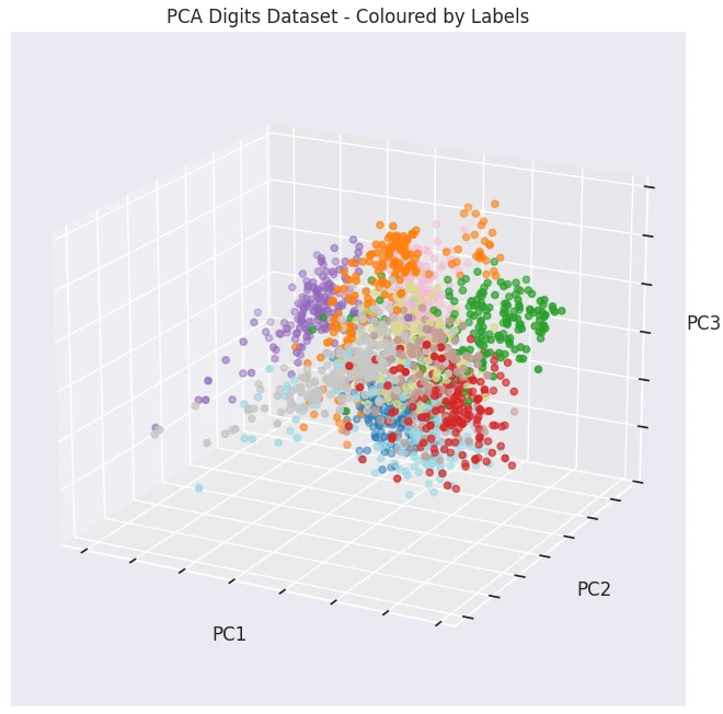
  • Dimensionality Reduction - Principal Component Analysis (PCA)
    • Dataset Preprocessing
    • Model Fitting
    • Dataset 2
      • Dataset 2 Preprocessing
      • Model Fitting

import matplotlib.pyplot as plt
import matplotlib.image as mpimg
from mpl_toolkits import mplot3d
import numpy as np
import pandas as pd
import plotly.express as px
from scipy.cluster import hierarchy
import seaborn as sns
from sklearn import svm
from sklearn.cluster import KMeans, AgglomerativeClustering, DBSCAN
from sklearn.datasets import load_iris, load_wine, fetch_20newsgroups, fetch_openml
from sklearn.impute import MissingIndicator, SimpleImputer
from sklearn.decomposition import PCA
from sklearn.ensemble import (
    RandomForestClassifier,
    RandomForestRegressor,
    GradientBoostingRegressor,
    AdaBoostRegressor,
    GradientBoostingClassifier,
    AdaBoostClassifier
)
from sklearn.feature_extraction.text import (
    CountVectorizer,
    TfidfTransformer,
    TfidfVectorizer
)
from sklearn.linear_model import (
    LinearRegression,
    LogisticRegression,
    Ridge,
    ElasticNet
)
from sklearn.metrics import (
    mean_absolute_error,
    mean_squared_error,
    classification_report,
    confusion_matrix,
    ConfusionMatrixDisplay,
    accuracy_score
)
from sklearn.model_selection import (
    train_test_split,
    GridSearchCV,
    cross_val_score,
    cross_validate
)
from sklearn.naive_bayes import MultinomialNB
from sklearn.neighbors import KNeighborsClassifier, KNeighborsRegressor
from sklearn.pipeline import Pipeline, make_pipeline
from sklearn.preprocessing import (
    MinMaxScaler,
    StandardScaler,
    OrdinalEncoder,
    LabelEncoder,
    OneHotEncoder,
    PolynomialFeatures
)
from sklearn.tree import DecisionTreeClassifier, DecisionTreeRegressor

Working with Missing Values

X_missing = pd.DataFrame(
    np.array([5,2,3,np.NaN,np.NaN,4,-3,2,1,8,np.NaN,4,10,np.NaN,5]).reshape(5,3)
)
X_missing.columns = ['f1','f2','f3']

X_missing

	f1	f2	f3
0	5.0	2.0	3.0
1	NaN	NaN	4.0
2	-3.0	2.0	1.0
3	8.0	NaN	4.0
4	10.0	NaN	5.0

X_missing.isnull().sum()

# f1    1
# f2    3
# f3    0
# dtype: int64

Missing Indicator

indicator = MissingIndicator(missing_values=np.NaN)
indicator = indicator.fit_transform(X_missing)
indicator = pd.DataFrame(indicator, columns=['a1', 'a2'])
indicator

	a1	a2
0	False	False
1	True	True
2	False	False
3	False	True
4	False	True

Simple Imputer

imputer_mean = SimpleImputer(missing_values=np.NaN, strategy='mean')
X_filled_mean = pd.DataFrame(imputer_mean.fit_transform(X_missing))
X_filled_mean.columns = ['f1','f2','f3']
X_filled_mean

	f1	f2	f3
0	5.0	2.0	3.0
1	5.0	2.0	4.0
2	-3.0	2.0	1.0
3	8.0	2.0	4.0
4	10.0	2.0	5.0

imputer_median = SimpleImputer(missing_values=np.NaN, strategy='median')
X_filled_median = pd.DataFrame(imputer_median.fit_transform(X_missing))
X_filled_median.columns = ['f1','f2','f3']
X_filled_median

	f1	f2	f3
0	5.0	2.0	3.0
1	6.5	2.0	4.0
2	-3.0	2.0	1.0
3	8.0	2.0	4.0
4	10.0	2.0	5.0

imputer_median = SimpleImputer(missing_values=np.NaN, strategy='most_frequent')
X_filled_median = pd.DataFrame(imputer_median.fit_transform(X_missing))
X_filled_median.columns = ['f1','f2','f3']
X_filled_median

	f1	f2	f3
0	5.0	2.0	3.0
1	-3.0	2.0	4.0
2	-3.0	2.0	1.0
3	8.0	2.0	4.0
4	10.0	2.0	5.0

Drop Missing Data

X_missing_dropped = X_missing.dropna(axis=1)
X_missing_dropped

	f3
0	3.0
1	4.0
2	1.0
3	4.0
4	5.0

X_missing_dropped = X_missing.dropna(axis=0).reset_index()
X_missing_dropped

	f1	f2	f3
0	5.0	2.0	3.0
1	-3.0	2.0	1.0

Categorical Data Preprocessing

X_cat_df = pd.DataFrame(
    np.array([
        ['M', 'O-', 'medium'],
        ['M', 'O-', 'high'],
        ['F', 'O+', 'high'],
        ['F', 'AB', 'low'],
        ['F', 'B+', 'medium']
    ])
)

X_cat_df.columns = ['f1','f2','f3']

X_cat_df

	f1	f2	f3
0	M	O-	medium
1	M	O-	high
2	F	O+	high
3	F	AB	low
4	F	B+	medium

Ordinal Encoder

encoder_ord = OrdinalEncoder(dtype='int')

X_cat_df.f3 = encoder_ord.fit_transform(X_cat_df.f3.values.reshape(-1, 1))
X_cat_df

	f1	f2	f3
0	M	O-	2
1	M	O-	0
2	F	O+	0
3	F	AB	1
4	F	B+	2

Label Encoder

encoder_lab = LabelEncoder()
X_cat_df['f2'] = encoder_lab.fit_transform(X_cat_df['f2'])
X_cat_df

	f1	f2	f3
0	M	3	2
1	M	3	0
2	F	2	0
3	F	0	1
4	F	1	2

OneHot Encoder

encoder_oh = OneHotEncoder(dtype='int')

onehot_df = pd.DataFrame(
    encoder_oh.fit_transform(X_cat_df[['f1']])
    .toarray(),
    columns=['F', 'M']
)

onehot_df['f2'] = X_cat_df.f2
onehot_df['f3'] = X_cat_df.f3
onehot_df

	F	M	f2	f3
0	0	1	3	2
1	0	1	3	0
2	1	0	2	0
3	1	0	0	1
4	1	0	1	2

Loading SK Datasets

Toy Datasets

load_iris(*[, return_X_y, as_frame])	classification	Load and return the iris dataset.
load_diabetes(*[, return_X_y, as_frame, scaled])	regression	Load and return the diabetes dataset.
load_digits(*[, n_class, return_X_y, as_frame])	classification	Load and return the digits dataset.
load_linnerud(*[, return_X_y, as_frame])	multi-output regression	Load and return the physical exercise Linnerud dataset.
load_wine(*[, return_X_y, as_frame])	classification	Load and return the wine dataset.
load_breast_cancer(*[, return_X_y, as_frame])	classification	Load and return the breast cancer wisconsin dataset.

iris_ds = load_iris()
iris_data = iris_ds.data
col_names = iris_ds.feature_names
target_names = iris_ds.target_names

print(
    'Iris Dataset',
    '\n * Data array: ',
    iris_data.shape,
    '\n * Column names: ',
    col_names,
    '\n * Target names: ',
    target_names
)

# Iris Dataset 
#  * Data array:  (150, 4) 
#  * Column names:  ['sepal length (cm)', 'sepal width (cm)', 'petal length (cm)', 'petal width (cm)'] 
#  * Target names:  ['setosa' 'versicolor' 'virginica']

iris_df = pd.DataFrame(data=iris_data, columns=col_names)

iris_df.head()

	sepal length (cm)	sepal width (cm)	petal length (cm)	petal width (cm)
0	5.1	3.5	1.4	0.2
1	4.9	3.0	1.4	0.2
2	4.7	3.2	1.3	0.2
3	4.6	3.1	1.5	0.2
4	5.0	3.6	1.4	0.2

Real World Datasets

fetch_olivetti_faces(*[, data_home, ...])	classification	Load the Olivetti faces data-set from AT&T.
fetch_20newsgroups(*[, data_home, subset, ...])	classification	Load the filenames and data from the 20 newsgroups dataset.
fetch_20newsgroups_vectorized(*[, subset, ...])	classification	Load and vectorize the 20 newsgroups dataset.
fetch_lfw_people(*[, data_home, funneled, ...])	classification	Load the Labeled Faces in the Wild (LFW) people dataset.
fetch_lfw_pairs(*[, subset, data_home, ...])	classification	Load the Labeled Faces in the Wild (LFW) pairs dataset.
fetch_covtype(*[, data_home, ...])	classification	Load the covertype dataset.
fetch_rcv1(*[, data_home, subset, ...])	classification	Load the RCV1 multilabel dataset.
fetch_kddcup99(*[, subset, data_home, ...])	classification	Load the kddcup99 dataset.
fetch_california_housing(*[, data_home, ...])	regression	Load the California housing dataset.

newsgroups_train = fetch_20newsgroups(subset='train')
train_data = newsgroups_train.data
col_names = newsgroups_train.filenames.shape
target_names = newsgroups_train.target.shape

print(
    'Newsgroup - Train Subset',
    '\n * Data array: ',
    len(train_data),
    '\n * Column names: ',
    col_names,
    '\n * Target names: ',
    target_names
)

# Newsgroup - Train Subset 
#  * Data array:  11314 
#  * Column names:  (11314,) 
#  * Target names:  (11314,)

print('Target Names: ', newsgroups_train.target_names)

# Target Names:  ['alt.atheism', 'comp.graphics', 'comp.os.ms-windows.misc', 'comp.sys.ibm.pc.hardware', 'comp.sys.mac.hardware', 'comp.windows.x', 'misc.forsale', 'rec.autos', 'rec.motorcycles', 'rec.sport.baseball', 'rec.sport.hockey', 'sci.crypt', 'sci.electronics', 'sci.med', 'sci.space', 'soc.religion.christian', 'talk.politics.guns', 'talk.politics.mideast', 'talk.politics.misc', 'talk.religion.misc']

OpenML Datasets

• openml.org
• Mice Protein Dataset

mice_ds = fetch_openml(name='miceprotein', version=4, parser="auto")

print(
    'Mice Protein Dataset',
    '\n * Data Shape: ',
    mice_ds.data.shape,
    '\n * Target Shape: ',
    mice_ds.target.shape,
    '\n * Target Names: ',
    np.unique(mice_ds.target)
)

# Mice Protein Dataset 
#  * Data Shape:  (1080, 77) 
#  * Target Shape:  (1080,) 
#  * Target Names:  ['c-CS-m' 'c-CS-s' 'c-SC-m' 'c-SC-s' 't-CS-m' 't-CS-s' 't-SC-m' 't-SC-s']

print(mice_ds.DESCR)

Supervised Learning - Regression Models

Simple Linear Regression

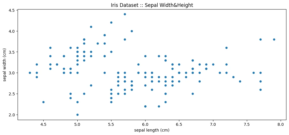
iris_df.plot(
    figsize=(12,5),
    kind='scatter',
    x='sepal length (cm)',
    y='sepal width (cm)',
    title='Iris Dataset :: Sepal Width&Height'
)

print(iris_df.corr())

The Sepal Width has very little correlation to all other metrics but itself. While the other three correlate nicely:

	sepal length (cm)	sepal width (cm)	petal length (cm)	petal width (cm)
sepal length (cm)	1.000000	-0.117570	0.871754	0.817941
sepal width (cm)	-0.117570	1.000000	-0.428440	-0.366126
petal length (cm)	0.871754	-0.428440	1.000000	0.962865
petal width (cm)	0.817941	-0.366126	0.962865	1.000000

Data Pre-processing

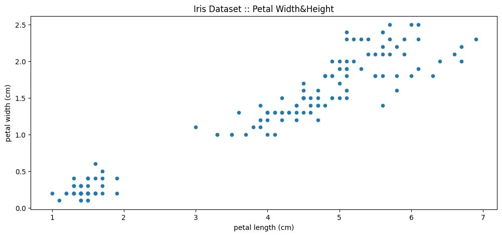
iris_df['petal length (cm)'][:1]
# 0    1.4
# Name: petal length (cm), dtype: float64

iris_df['petal length (cm)'].values.reshape(-1,1)[:1]
# array([[1.4]])

# scikit expects a 2s imput => remove index
X = iris_df['petal length (cm)'].values.reshape(-1,1)
y = iris_df['petal width (cm)'].values.reshape(-1,1)

# train/test split
X_train, X_test, y_train, y_test = train_test_split(X,y,test_size=0.2)
print(X_train.shape, X_test.shape)
# (120, 1) (30, 1) 80:20 split

Model Training

regressor = LinearRegression()
regressor.fit(X_train,y_train)

intercept = regressor.intercept_
slope = regressor.coef_

print(' Intercept: ', intercept, '\n Slope: ', slope)
#  Intercept:  [-0.35135666] 
#  Correlation Coeficient:  [[0.41310505]]

Predictions

y_pred = regressor.predict([X_test[0]])
print(' Prediction: ', y_pred, '\n True Value: ', y_test[0])
#  Prediction:  [[0.22699041]] 
#  True Value:  [0.2]

def predict(value):
    return (slope*value + intercept)[0][0]

print('Prediction: ', predict(X_test[0]))
# Prediction:  [[0.22699041]]

iris_df['petal width (cm) prediction'] = iris_df['petal length (cm)'].apply(predict)
print(' Prediction: ', iris_df['petal width (cm) prediction'][0], '\n True Value: ', iris_df['petal width (cm)'][0])
#  Prediction:  0.22699041280334376 
#  True Value:  0.2

iris_df.head(10)

	sepal length (cm)	sepal width (cm)	petal length (cm)	petal width (cm)	petal width (cm) prediction
0	5.1	3.5	1.4	0.2	0.226990
1	4.9	3.0	1.4	0.2	0.226990
2	4.7	3.2	1.3	0.2	0.185680
3	4.6	3.1	1.5	0.2	0.268301
4	5.0	3.6	1.4	0.2	0.226990
5	5.4	3.9	1.7	0.4	0.350922
6	4.6	3.4	1.4	0.3	0.226990
7	5.0	3.4	1.5	0.2	0.268301
8	4.4	2.9	1.4	0.2	0.226990
9	4.9	3.1	1.5	0.1	0.268301

iris_df.plot(
    figsize=(12,5),
    kind='scatter',
    x='petal width (cm)',
    y='petal width (cm) prediction',
    # no value in colorizing..just looks pretty
    c='petal width (cm) prediction',
    colormap='summer',
    title='Iris Dataset - Sepal Width True vs Prediction'
)

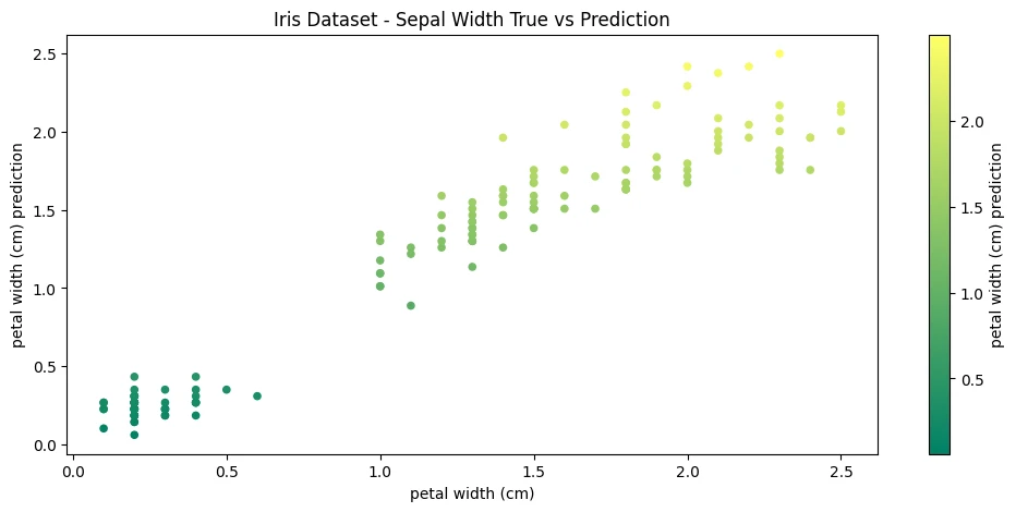
Model Evaluation

mae = mean_absolute_error(
    iris_df['petal width (cm)'],
    iris_df['petal width (cm) prediction']
)

mse = mean_squared_error(
    iris_df['petal width (cm)'],
    iris_df['petal width (cm) prediction']
)

rmse = np.sqrt(mse)

print(' MAE: ', mae, '\n MSE: ', mse, '\n RMSE: ', rmse)

#  MAE:  0.1569441318761155 
#  MSE:  0.04209214667485277 
#  RMSE:  0.2051637070118708

ElasticNet Regression

Dataset

!wget https://raw.githubusercontent.com/Satish-Vennapu/DataScience/main/AMES_Final_DF.csv -P datasets

ames_df = pd.read_csv('datasets/AMES_Final_DF.csv')
ames_df.head(5).transpose()

	0	1	2	3	4
Lot Frontage	141.0	80.0	81.0	93.0	74.0
Lot Area	31770.0	11622.0	14267.0	11160.0	13830.0
Overall Qual	6.0	5.0	6.0	7.0	5.0
Overall Cond	5.0	6.0	6.0	5.0	5.0
Year Built	1960.0	1961.0	1958.0	1968.0	1997.0
...
Sale Condition_AdjLand	0.0	0.0	0.0	0.0	0.0
Sale Condition_Alloca	0.0	0.0	0.0	0.0	0.0
Sale Condition_Family	0.0	0.0	0.0	0.0	0.0
Sale Condition_Normal	1.0	1.0	1.0	1.0	1.0
Sale Condition_Partial	0.0	0.0	0.0	0.0	0.0
274 rows × 5 columns

# the target value is:
ames_df['SalePrice']

0	215000
1	105000
2	172000
3	244000
4	189900
...
2920	142500
2921	131000
2922	132000
2923	170000
2924	188000
Name: SalePrice, Length: 2925, dtype: int64

Preprocessing

# remove target column from training dataset
X_ames = ames_df.drop('SalePrice', axis=1)
y_ames = ames_df['SalePrice']

print(X_ames.shape, y_ames.shape)
# (2925, 273) (2925,)

# train/test split
X_ames_train, X_ames_test, y_ames_train, y_ames_test = train_test_split(
    X_ames,
    y_ames,
    test_size=0.1,
    random_state=101
)

print(X_ames_train.shape, X_ames_test.shape)
# (2632, 273) (293, 273)

# normalize feature set
scaler = StandardScaler()
X_ames_train_scaled = scaler.fit_transform(X_ames_train)

X_ames_test_scaled = scaler.transform(X_ames_test)

Grid Search for Hyperparameters

base_ames_elastic_net_model = ElasticNet(max_iter=int(1e4))

param_grid = \{
    'alpha': [50, 75, 100, 125, 150],
    'l1_ratio':[0.2, 0.4, 0.6, 0.8, 1.0]
\}

grid_ames_model = GridSearchCV(
    estimator=base_ames_elastic_net_model,
    param_grid=param_grid,
    scoring='neg_mean_squared_error',
    cv=5, verbose=1
)

grid_ames_model.fit(X_ames_train_scaled, y_ames_train)

print(
    'Results:\nBest Estimator: ',
    grid_ames_model.best_estimator_,
    '\nBest Hyperparameter: ',
    grid_ames_model.best_params_
)

Results:

• Best Estimator: ElasticNet(alpha=125, l1_ratio=1.0, max_iter=10000)
• Best Hyperparameter: \{'alpha': 125, 'l1_ratio': 1.0\}

Model Evaluation

y_ames_pred = grid_ames_model.predict(X_ames_test_scaled)

print(
    'MAE: ',
    mean_absolute_error(y_ames_test, y_ames_pred),
    'MSE: ',
    mean_squared_error(y_ames_test, y_ames_pred),
    'RMSE: ',
    np.sqrt(mean_squared_error(y_ames_test, y_ames_pred))
)

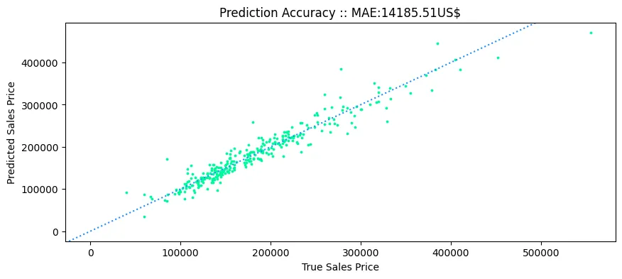
# MAE:  14185.506207185055 MSE:  422714457.5190704 RMSE:  20560.020854052418

# average SalePrize
np.mean(ames_df['SalePrice'])
# 180815.53743589742

rel_error_avg = mean_absolute_error(y_ames_test, y_ames_pred) * 100 / np.mean(ames_df['SalePrice'])
print('Pridictions are on average off by: ', rel_error_avg.round(2), '%')
# Pridictions are on average off by:  7.85 %

plt.figure(figsize=(10,4))

plt.scatter(y_ames_test,y_ames_pred, c='mediumspringgreen', s=3)
plt.axline((0, 0), slope=1, color='dodgerblue', linestyle=(':'))

plt.title('Prediction Accuracy :: MAE:'+ str(mean_absolute_error(y_ames_test, y_ames_pred).round(2)) + 'US$')
plt.xlabel('True Sales Price')
plt.ylabel('Predicted Sales Price')
plt.savefig('assets/Scikit_Learn_11.webp', bbox_inches='tight')

Multiple Linear Regression

Above I used the petal width and length to create a linear regression model. But as explored earlier we can also use the sepal length (only the sepal width does not show a linear correlation):

print(iris_df.corr())

	sepal length (cm)	sepal width (cm)	petal length (cm)	petal width (cm)
sepal length (cm)	1.000000	-0.117570	0.871754	0.817941
sepal width (cm)	-0.117570	1.000000	-0.428440	-0.366126
petal length (cm)	0.871754	-0.428440	1.000000	0.962865
petal width (cm)	0.817941	-0.366126	0.962865	1.000000

X_multi = iris_df[['petal length (cm)', 'sepal length (cm)']]
y = iris_df['petal width (cm)']

regressor_multi = LinearRegression()
regressor_multi.fit(X_multi, y)

intercept_multi = regressor_multi.intercept_
slope_multi = regressor_multi.coef_

print(' Intercept: ', intercept_multi, '\n Slope: ', slope_multi)

#  Intercept:  -0.00899597269816943 
#  Slope:  [ 0.44937611 -0.08221782]

def predict_multi(petal_length, sepal_length):
    return (slope_multi[0]*petal_length + slope_multi[1]*sepal_length + intercept_multi)

y_pred = predict_multi(
    iris_df['petal length (cm)'][0],
    iris_df['sepal length (cm)'][0]
)

print(' Prediction: ', y_pred, '\n True value: ', iris_df['petal width (cm)'][0])
#  Prediction:  0.20081970121763193 
#  True value:  0.2

iris_df['petal width (cm) prediction (multi)'] = (
    (
        slope_multi[0] * iris_df['petal length (cm)']
    ) + (
        slope_multi[1] * iris_df['sepal length (cm)']
    ) + (
        intercept_multi
    ) 
)

iris_df.head(10)

	sepal length (cm)	sepal width (cm)	petal length (cm)	petal width (cm)	petal width (cm) prediction	petal width (cm) prediction (multi)
0	5.1	3.5	1.4	0.2	0.226990	0.200820
1	4.9	3.0	1.4	0.2	0.226990	0.217263
2	4.7	3.2	1.3	0.2	0.185680	0.188769
3	4.6	3.1	1.5	0.2	0.268301	0.286866
4	5.0	3.6	1.4	0.2	0.226990	0.209041
5	5.4	3.9	1.7	0.4	0.350922	0.310967
6	4.6	3.4	1.4	0.3	0.226990	0.241929
7	5.0	3.4	1.5	0.2	0.268301	0.253979
8	4.4	2.9	1.4	0.2	0.226990	0.258372
9	4.9	3.1	1.5	0.1	0.268301	0.262201

iris_df.plot(
    figsize=(12,5),
    kind='scatter',
    x='petal width (cm)',
    y='petal width (cm) prediction (multi)',
    c='petal width (cm) prediction',
    colormap='summer',
    title='Iris Dataset - Sepal Width True vs Prediction (multi)'
)

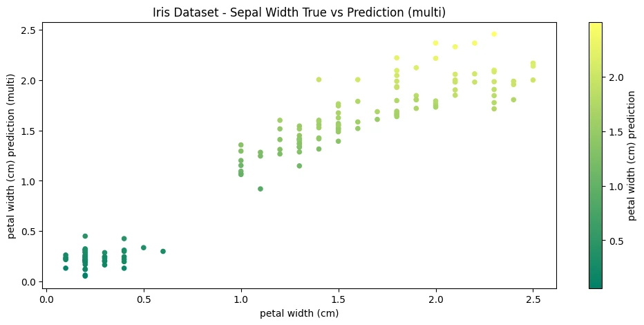
mae_multi = mean_absolute_error(
    iris_df['petal width (cm)'],
    iris_df['petal width (cm) prediction (multi)']
)

mse_multi = mean_squared_error(
    iris_df['petal width (cm)'],
    iris_df['petal width (cm) prediction (multi)']
)

rmse_multi = np.sqrt(mse_multi)

print(' MAE_Multi: ', mae_multi,' MAE: ', mae, '\n MSE_Multi: ', mse_multi, ' MSE: ', mse, '\n RMSE_Multi: ', rmse_multi, ' RMSE: ', rmse)

The accuracy of the model was improved by adding an additional, correlating value:

	Multi Regression	Single Regression
Mean Absolute Error	0.15562108079300102	0.1569441318761155
Mean Squared Error	0.04096208526408982	0.04209214667485277
Root Mean Squared Error	0.20239092189149646	0.2051637070118708

Supervised Learning - Logistic Regression Model

Binary Logistic Regression

Dataset

np.random.seed(666)

# generate 10 index values between 0-10
x_data_logistic_binary = np.random.randint(10, size=(10)).reshape(-1, 1)
# generate binary category for values above
y_data_logistic_binary = np.random.randint(2, size=10)

Model Fitting

logistic_binary_model = LogisticRegression(
    solver='liblinear',
    C=10.0,
    random_state=0
)

logistic_binary_model.fit(x_data_logistic_binary, y_data_logistic_binary)

intercept_logistic_binary = logistic_binary_model.intercept_
slope_logistic_binary = logistic_binary_model.coef_

print(' Intercept: ', intercept_logistic_binary, '\n Slope: ', slope_logistic_binary)

#  Intercept:  [-0.4832956] 
#  Slope:  [[0.11180522]]

Model Predictions

prob_pred_logistic_binary = logistic_binary_model.predict_proba(x_data_logistic_binary)
y_pred_logistic_binary = logistic_binary_model.predict(x_data_logistic_binary)


print('Prediction Probabilities: ', prob_pred[:1])

unique, counts = np.unique(y_pred_logistic_binary, return_counts=True)
print('Classes: ', unique, '| Number of Class Instances: ', counts)

# probabilities e.g. below -> 58% certainty that the first element is class 0

# Prediction Probabilities:  [[0.58097284 0.41902716]]
# Classes:  [0 1] | Number of Class Instances:  [5 5]

Model Evaluation

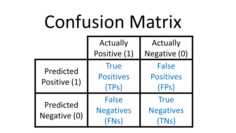
conf_mtx = confusion_matrix(y_data_logistic_binary, y_pred_logistic_binary)
conf_mtx

# [2, 3] [TP, FP]
# [3, 2] [FN, TN]

report = classification_report(y_data_logistic_binary, y_pred_logistic_binary)
print(report)

	precision	recall	f1-score	support
0	0.40	0.40	0.40	5
1	0.40	0.40	0.40	5
accuracy			0.40	10
macro avg	0.40	0.40	0.40	10
weighted avg	0.40	0.40	0.40	10

Logistic Regression Pipelines

Dataset Preprocessing

iris_ds = load_iris()

# train/test split
X_train_iris, X_test_iris, y_train_iris, y_test_iris = train_test_split(
    iris_ds.data,
    iris_ds.target,
    test_size=0.2,
    random_state=42
)
print(X_train_iris.shape, X_test_iris.shape)
# (120, 4) (30, 4)

Pipeline

pipe_iris = Pipeline([
    ('minmax', MinMaxScaler()),
    ('log_reg', LogisticRegression()),
])

pipe_iris.fit(X_train_iris, y_train_iris)

iris_score = pipe_iris.score(X_test_iris, y_test_iris)
print('Prediction Accuracy: ', iris_score.round(4)*100, '%')
# Prediction Accuracy:  96.67 %

Cross Validation

Train | Test Split

!wget https://raw.githubusercontent.com/reisanar/datasets/master/Advertising.csv -P datasets

adv_df = pd.read_csv('datasets/Advertising.csv')
adv_df.head(5)

	TV	Radio	Newspaper	Sales
0	230.1	37.8	69.2	22.1
1	44.5	39.3	45.1	10.4
2	17.2	45.9	69.3	9.3
3	151.5	41.3	58.5	18.5
4	180.8	10.8	58.4	12.9

# Split ds into features and targets
X_adv = adv_df.drop('Sales', axis=1)
y_adv = adv_df['Sales']

# 70:30 train/test split
X_adv_train, X_adv_test, y_adv_train, y_adv_test = train_test_split(
    X_adv, y_adv, test_size=0.3, random_state=666
)

print(X_adv_train.shape, y_adv_train.shape)
# (140, 3) (140,)

# normalize features
scaler_adv = StandardScaler()
scaler_adv.fit(X_adv_train)

X_adv_train = scaler_adv.transform(X_adv_train)
X_adv_test = scaler_adv.transform(X_adv_test)

Model Fitting

model_adv1 = Ridge(
    alpha=100.0
)

model_adv1.fit(X_adv_train, y_adv_train)

Model Evaluation

y_adv_pred = model_adv1.predict(X_adv_test)

mean_squared_error(y_adv_test, y_adv_pred)
# 6.528575771818745

Adjusting Hyper Parameter

model_adv2 = Ridge(
    alpha=1.0
)

model_adv2.fit(X_adv_train, y_adv_train)

y_adv_pred2 = model_adv2.predict(X_adv_test)
mean_squared_error(y_adv_test, y_adv_pred2)
# 2.3319016551123535

Train | Validation | Test Split

# 70:30 train/temp split
X_adv_train, X_adv_temp, y_adv_train, y_adv_temp = train_test_split(
    X_adv, y_adv, test_size=0.3, random_state=666
)

# 50:50 test/val split
X_adv_test, X_adv_val, y_adv_test, y_adv_val = train_test_split(
    X_adv_temp, y_adv_temp, test_size=0.5, random_state=666
)

print(X_adv_train.shape, X_adv_test.shape, X_adv_val.shape)
# (140, 3) (30, 3) (30, 3)

# normalize features
scaler_adv = StandardScaler()
scaler_adv.fit(X_adv_train)

X_adv_train = scaler_adv.transform(X_adv_train)
X_adv_test = scaler_adv.transform(X_adv_test)
X_adv_val = scaler_adv.transform(X_adv_val)

Model Fitting and Evaluation

model_adv3 = Ridge(
    alpha=100.0
)

model_adv3.fit(X_adv_train, y_adv_train)

# do evaluation with the validation set
y_adv_pred3 = model_adv3.predict(X_adv_val)
mean_squared_error(y_adv_val, y_adv_pred3)
# 7.136230975501291

Adjusting Hyper Parameter

model_adv4 = Ridge(
    alpha=1.0
)

model_adv4.fit(X_adv_train, y_adv_train)

y_adv_pred4 = model_adv4.predict(X_adv_val)
mean_squared_error(y_adv_val, y_adv_pred4)
# 2.6393803874124435

# only once you are certain that you have the best performance
# do a final evaluation with the test set
y_adv4_final_pred = model_adv4.predict(X_adv_test)
mean_squared_error(y_adv_test, y_adv4_final_pred)
# 2.024422922812264

k-fold Cross Validation

Do a train/test split and segment the training set by k-folds (e.g. 5-10) and use each of those segments once to validate a training step. The resulting error is the average of all k errors.

Train-Test Split

# 70:30 train/temp split
X_adv_train, X_adv_test, y_adv_train, y_adv_test = train_test_split(
    X_adv, y_adv, test_size=0.3, random_state=666
)

# normalize features
scaler_adv = StandardScaler()
scaler_adv.fit(X_adv_train)

X_adv_train = scaler_adv.transform(X_adv_train)
X_adv_test = scaler_adv.transform(X_adv_test)

Model Scoring

model_adv5 = Ridge(
    alpha=100.0
)

# do a 5-fold cross-eval
scores = cross_val_score(
    estimator=model_adv5,
    X=X_adv_train,
    y=y_adv_train,
    scoring='neg_mean_squared_error',
    cv=5
)

# take the mean of all five neg. error values
abs(scores.mean())
# 8.688107513529168

Adjusting Hyper Parameter

model_adv6 = Ridge(
    alpha=1.0
)

# do a 5-fold cross-eval
scores = cross_val_score(
    estimator=model_adv6,
    X=X_adv_train,
    y=y_adv_train,
    scoring='neg_mean_squared_error',
    cv=5
)

# take the mean of all five neg. error values
abs(scores.mean())
# 3.3419582340688576

Model Fitting and Final Evaluation

model_adv6.fit(X_adv_train, y_adv_train)

y_adv6_final_pred = model_adv6.predict(X_adv_test)
mean_squared_error(y_adv_test, y_adv6_final_pred)
# 2.3319016551123535

Cross Validate

Dataset (re-import)

adv_df = pd.read_csv('datasets/Advertising.csv')
X_adv = adv_df.drop('Sales', axis=1)
y_adv = adv_df['Sales']

# 70:30 train/test split
X_adv_train, X_adv_test, y_adv_train, y_adv_test = train_test_split(
    X_adv, y_adv, test_size=0.3, random_state=666
)

# normalize features
scaler_adv = StandardScaler()
scaler_adv.fit(X_adv_train)

X_adv_train = scaler_adv.transform(X_adv_train)
X_adv_test = scaler_adv.transform(X_adv_test)

Model Scoring

model_adv7 = Ridge(
    alpha=100.0
)

scores = cross_validate(
    model_adv7,
    X_adv_train,
    y_adv_train,
    scoring=[
        'neg_mean_squared_error',
        'neg_mean_absolute_error'
    ],
    cv=10
)

scores_df = pd.DataFrame(scores)
scores_df

	fit_time	score_time	test_neg_mean_squared_error	test_neg_mean_absolute_error
0	0.016399	0.000749	-12.539147	-2.851864
1	0.000684	0.000452	-2.806466	-1.423516
2	0.000937	0.000782	-11.142227	-2.740332
3	0.001060	0.000633	-7.237347	-2.196963
4	0.001045	0.000738	-11.313985	-2.690813
5	0.000650	0.000510	-3.169169	-1.526568
6	0.000698	0.000429	-6.578249	-1.727616
7	0.000600	0.000423	-5.740245	-1.640964
8	0.000565	0.000463	-10.268075	-2.415688
9	0.000562	0.000487	-10.641669	-1.974407

abs(scores_df.mean())

fit_time	0.002320
score_time	0.000566
test_neg_mean_squared_error	8.143658
test_neg_mean_absolute_error	2.118873
dtype: float64

Adjusting Hyper Parameter

model_adv8 = Ridge(
    alpha=1.0
)

scores = cross_validate(
    model_adv8,
    X_adv_train,
    y_adv_train,
    scoring=[
        'neg_mean_squared_error',
        'neg_mean_absolute_error'
    ],
    cv=10
)

abs(pd.DataFrame(scores).mean())

fit_time	0.001141
score_time	0.000777
test_neg_mean_squared_error	3.272673
test_neg_mean_absolute_error	1.345709
dtype: float64

Model Fitting and Final Evaluation

model_adv8.fit(X_adv_train, y_adv_train)

y_adv8_final_pred = model_adv8.predict(X_adv_test)
mean_squared_error(y_adv_test, y_adv8_final_pred)
# 2.3319016551123535

Grid Search

Loop through a set of hyperparameters to find an optimum.

Hyperparameter Search

base_elastic_net_model = ElasticNet()

param_grid = \{
    'alpha': [0.1, 1, 5, 10, 50, 100],
    'l1_ratio':[0.1, 0.3, 0.5, 0.7, 0.9, 1.0]
\}

grid_model = GridSearchCV(
    estimator=base_elastic_net_model,
    param_grid=param_grid,
    scoring='neg_mean_squared_error',
    cv=5, verbose=2
)

grid_model.fit(X_adv_train, y_adv_train)

print(
    'Results:\nBest Estimator: ',
    grid_model.best_estimator_,
    '\nBest Hyperparameter: ',
    grid_model.best_params_
)

Results:

• Best Estimator: ElasticNet(alpha=0.1, l1_ratio=1.0)
• Best Hyperparameter: \{'alpha': 0.1, 'l1_ratio': 1.0\}

gridcv_results = pd.DataFrame(grid_model.cv_results_)

	mean_fit_time	std_fit_time	mean_score_time	std_score_time	param_alpha	param_l1_ratio	params	split0_test_score	split1_test_score	split2_test_score	split3_test_score	split4_test_score	mean_test_score	std_test_score	rank_test_score
0	0.001156	0.000160	0.000449	0.000038	0.1	0.1	{'alpha': 0.1, 'l1_ratio': 0.1}	-1.924119	-3.384152	-3.588444	-3.703040	-5.091974	-3.538346	1.007264	6
1	0.001144	0.000181	0.000407	0.000091	0.1	0.3	{'alpha': 0.1, 'l1_ratio': 0.3}	-1.867117	-3.304382	-3.561106	-3.623188	-5.061781	-3.483515	1.016000	5
2	0.000623	0.000026	0.000272	0.000052	0.1	0.5	{'alpha': 0.1, 'l1_ratio': 0.5}	-1.812633	-3.220727	-3.539711	-3.547572	-5.043259	-3.432780	1.028406	4
3	0.000932	0.000165	0.000321	0.000060	0.1	0.7	{'alpha': 0.1, 'l1_ratio': 0.7}	-1.750153	-3.144120	-3.525226	-3.477228	-5.034008	-3.386147	1.046722	3
4	0.000725	0.000106	0.000259	0.000024	0.1	0.9	{'alpha': 0.1, 'l1_ratio': 0.9}	-1.693440	-3.075686	-3.518777	-3.413393	-5.029683	-3.346196	1.065195	2
5	0.000654	0.000053	0.000274	0.000026	0.1	1.0	{'alpha': 0.1, 'l1_ratio': 1.0}	-1.667506	-3.044928	-3.518866	-3.384363	-5.031297	-3.329392	1.075006	1
6	0.000595	0.000016	0.000244	0.000002	1	0.1	{'alpha': 1, 'l1_ratio': 0.1}	-8.575470	-11.021534	-8.212152	-6.808719	-10.792072	-9.081990	1.604192	12
7	0.000591	0.000018	0.000244	0.000002	1	0.3	{'alpha': 1, 'l1_ratio': 0.3}	-8.131855	-10.448423	-7.774620	-6.179358	-10.071728	-8.521197	1.569173	11
8	0.000628	0.000049	0.000266	0.000023	1	0.5	{'alpha': 1, 'l1_ratio': 0.5}	-7.519809	-9.562473	-7.261824	-5.453399	-9.213320	-7.802165	1.481785	10
9	0.000594	0.000015	0.000243	0.000002	1	0.7	{'alpha': 1, 'l1_ratio': 0.7}	-6.614835	-8.351711	-6.702104	-4.698977	-8.230616	-6.919649	1.329741	9
10	0.000714	0.000108	0.000268	0.000033	1	0.9	{'alpha': 1, 'l1_ratio': 0.9}	-5.537250	-6.887828	-6.148400	-4.106124	-7.101573	-5.956235	1.078430	8
11	0.000649	0.000067	0.000263	0.000028	1	1.0	{'alpha': 1, 'l1_ratio': 1.0}	-4.932027	-6.058207	-5.892529	-3.798441	-6.472871	-5.430815	0.959804	7
12	0.000645	0.000042	0.000264	0.000040	5	0.1	{'alpha': 5, 'l1_ratio': 0.1}	-21.863798	-25.767488	-18.768865	-12.608680	-23.207907	-20.443347	4.520904	13
13	0.000617	0.000030	0.000281	0.000038	5	0.3	{'alpha': 5, 'l1_ratio': 0.3}	-23.626694	-27.439028	-20.266203	-12.788078	-24.609195	-21.745840	5.031493	14
14	0.000599	0.000011	0.000249	0.000013	5	0.5	{'alpha': 5, 'l1_ratio': 0.5}	-26.202964	-29.867138	-22.527913	-13.423857	-26.835934	-23.771561	5.675911	15
15	0.000588	0.000013	0.000276	0.000035	5	0.7	{'alpha': 5, 'l1_ratio': 0.7}	-27.768946	-33.428462	-23.506474	-14.599984	-29.112276	-25.683228	6.382379	17
16	0.000580	0.000003	0.000271	0.000001	5	0.9	{'alpha': 5, 'l1_ratio': 0.9}	-29.868949	-34.423737	-25.623955	-16.750237	-31.056181	-27.544612	6.087093	19
17	0.000591	0.000011	0.000259	0.000021	5	1.0	{'alpha': 5, 'l1_ratio': 1.0}	-29.868949	-34.423737	-25.623955	-16.750237	-31.056181	-27.544612	6.087093	19
18	0.000632	0.000028	0.000250	0.000012	10	0.1	{'alpha': 10, 'l1_ratio': 0.1}	-26.179546	-30.396420	-22.386698	-14.596498	-27.292337	-24.170300	5.429322	16
19	0.000593	0.000020	0.000239	0.000001	10	0.3	{'alpha': 10, 'l1_ratio': 0.3}	-28.704426	-33.379967	-24.561645	-15.634153	-29.883725	-26.432783	6.090062	18
20	0.000595	0.000036	0.000245	0.000013	10	0.5	{'alpha': 10, 'l1_ratio': 0.5}	-29.868949	-34.423737	-25.623955	-16.750237	-31.056181	-27.544612	6.087093	19
21	0.000610	0.000053	0.000258	0.000015	10	0.7	{'alpha': 10, 'l1_ratio': 0.7}	-29.868949	-34.423737	-25.623955	-16.750237	-31.056181	-27.544612	6.087093	19
22	0.000597	0.000022	0.000248	0.000015	10	0.9	{'alpha': 10, 'l1_ratio': 0.9}	-29.868949	-34.423737	-25.623955	-16.750237	-31.056181	-27.544612	6.087093	19
23	0.000623	0.000057	0.000305	0.000076	10	1.0	{'alpha': 10, 'l1_ratio': 1.0}	-29.868949	-34.423737	-25.623955	-16.750237	-31.056181	-27.544612	6.087093	19
24	0.000602	0.000016	0.000252	0.000013	50	0.1	{'alpha': 50, 'l1_ratio': 0.1}	-29.868949	-34.423737	-25.623955	-16.750237	-31.056181	-27.544612	6.087093	19
25	0.000577	0.000009	0.000238	0.000001	50	0.3	{'alpha': 50, 'l1_ratio': 0.3}	-29.868949	-34.423737	-25.623955	-16.750237	-31.056181	-27.544612	6.087093	19
26	0.000607	0.000046	0.000245	0.000010	50	0.5	{'alpha': 50, 'l1_ratio': 0.5}	-29.868949	-34.423737	-25.623955	-16.750237	-31.056181	-27.544612	6.087093	19
27	0.000569	0.000004	0.000259	0.000012	50	0.7	{'alpha': 50, 'l1_ratio': 0.7}	-29.868949	-34.423737	-25.623955	-16.750237	-31.056181	-27.544612	6.087093	19
28	0.000582	0.000022	0.000244	0.000011	50	0.9	{'alpha': 50, 'l1_ratio': 0.9}	-29.868949	-34.423737	-25.623955	-16.750237	-31.056181	-27.544612	6.087093	19
29	0.000603	0.000041	0.000251	0.000015	50	1.0	{'alpha': 50, 'l1_ratio': 1.0}	-29.868949	-34.423737	-25.623955	-16.750237	-31.056181	-27.544612	6.087093	19
30	0.000670	0.000106	0.000251	0.000013	100	0.1	{'alpha': 100, 'l1_ratio': 0.1}	-29.868949	-34.423737	-25.623955	-16.750237	-31.056181	-27.544612	6.087093	19
31	0.000764	0.000179	0.000343	0.000054	100	0.3	{'alpha': 100, 'l1_ratio': 0.3}	-29.868949	-34.423737	-25.623955	-16.750237	-31.056181	-27.544612	6.087093	19
32	0.000623	0.000077	0.000244	0.000007	100	0.5	{'alpha': 100, 'l1_ratio': 0.5}	-29.868949	-34.423737	-25.623955	-16.750237	-31.056181	-27.544612	6.087093	19
33	0.000817	0.000156	0.000329	0.000076	100	0.7	{'alpha': 100, 'l1_ratio': 0.7}	-29.868949	-34.423737	-25.623955	-16.750237	-31.056181	-27.544612	6.087093	19
34	0.000590	0.000017	0.000242	0.000004	100	0.9	{'alpha': 100, 'l1_ratio': 0.9}	-29.868949	-34.423737	-25.623955	-16.750237	-31.056181	-27.544612	6.087093	19
35	0.000595	0.000027	0.000242	0.000007	100	1.0	{'alpha': 100, 'l1_ratio': 1.0}	-29.868949	-34.423737	-25.623955	-16.750237	-31.056181	-27.544612	6.087093	19

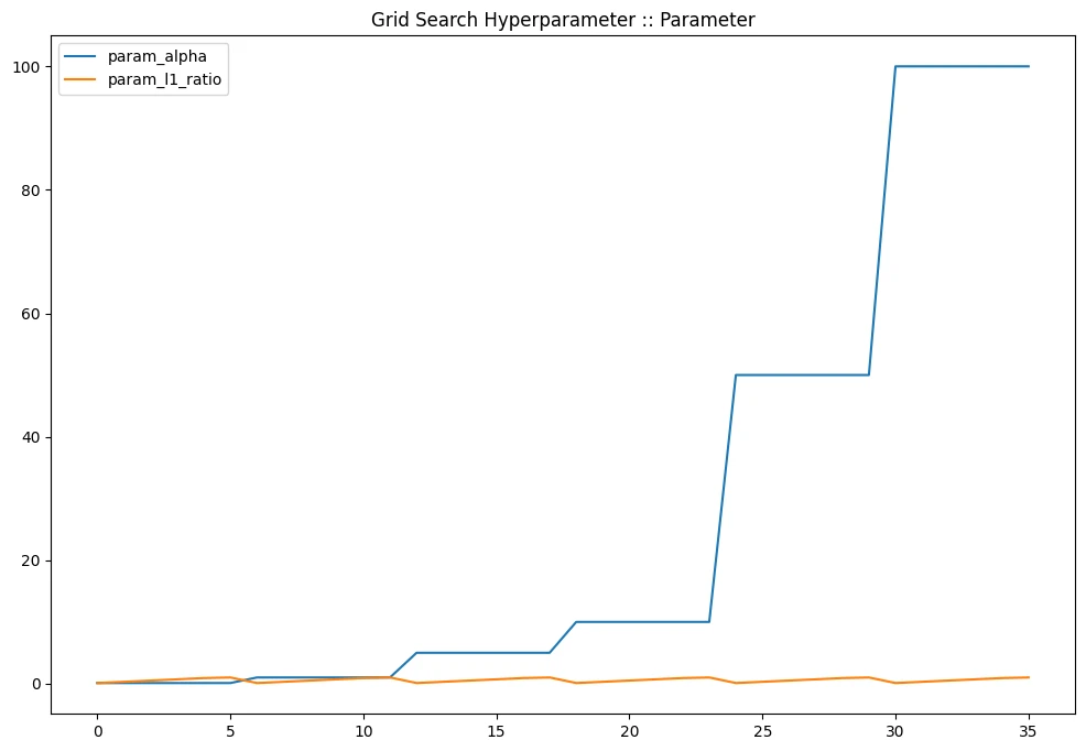
gridcv_results[
    [
        'param_alpha',
        'param_l1_ratio'
    ]
].plot(title='Grid Search Hyperparameter :: Parameter', figsize=(12,8))

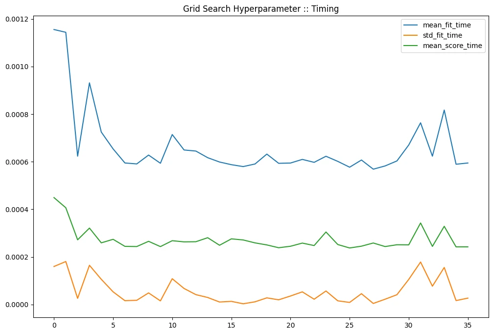
gridcv_results[
    [
        'mean_fit_time',
        'std_fit_time',
        'mean_score_time'
    ]
].plot(title='Grid Search Hyperparameter :: Timing', figsize=(12,8))

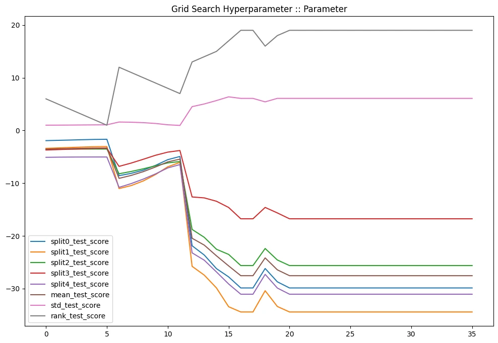
gridcv_results[
    [
        'split0_test_score',
        'split1_test_score',
        'split2_test_score',
        'split3_test_score',
        'split4_test_score',
        'mean_test_score',
        'std_test_score',
       'rank_test_score'
    ]
].plot(title='Grid Search Hyperparameter :: Parameter', figsize=(12,8))

Model Evaluation

y_grid_pred = grid_model.predict(X_adv_test)

mean_squared_error(y_adv_test, y_grid_pred)
# 2.380865536033581

Supervised Learning - KNN Algorithm

Dataset

wine = load_wine()
print(wine.data.shape)
print(wine.feature_names)
print(wine.data[:1])

# (178, 13)
# ['alcohol', 'malic_acid', 'ash', 'alcalinity_of_ash', 'magnesium', 'total_phenols', 'flavanoids', 'nonflavanoid_phenols', 'proanthocyanins', 'color_intensity', 'hue', 'od280/od315_of_diluted_wines', 'proline']
# [[1.423e+01 1.710e+00 2.430e+00 1.560e+01 1.270e+02 2.800e+00 3.060e+00
#   2.800e-01 2.290e+00 5.640e+00 1.040e+00 3.920e+00 1.065e+03]]

wine_df = pd.DataFrame(data=wine.data, columns=wine.feature_names)
wine_df.head(2).T

	0	1
alcohol	14.23	13.20
malic_acid	1.71	1.78
ash	2.43	2.14
alcalinity_of_ash	15.60	11.20
magnesium	127.00	100.00
total_phenols	2.80	2.65
flavanoids	3.06	2.76
nonflavanoid_phenols	0.28	0.26
proanthocyanins	2.29	1.28
color_intensity	5.64	4.38
hue	1.04	1.05
od280/od315_of_diluted_wines	3.92	3.40
proline	1065.00	1050.00

Data Pre-processing

# normalization
scaler = MinMaxScaler()
scaler.fit(wine.data)
wine_norm = scaler.fit_transform(wine.data)

# train/test split
X_train_wine, X_test_wine, y_train_wine, y_test_wine = train_test_split(
    wine_norm,
    wine.target,
    test_size=0.3
)

print(X_train_wine.shape, X_test_wine.shape)
# (124, 13) (54, 13)

Model Fitting

# model for k=3
knn = KNeighborsClassifier(n_neighbors=3)
knn.fit(X_train_wine, y_train_wine)

y_pred_wine_knn3 = knn.predict(X_test_wine)
print('Accuracy Score: ', (accuracy_score(y_test_wine, y_pred_wine_knn3)*100).round(2), '%')
# Accuracy Score:  98.15 %

# model for k=5
knn = KNeighborsClassifier(n_neighbors=5)
knn.fit(X_train_wine, y_train_wine)

y_pred_wine_knn5 = knn.predict(X_test_wine)
print('Accuracy Score: ', (accuracy_score(y_test_wine, y_pred_wine_knn5)*100).round(2), '%')
# Accuracy Score:  98.15 %

# model for k=7
knn = KNeighborsClassifier(n_neighbors=7)
knn.fit(X_train_wine, y_train_wine)

y_pred_wine_knn7 = knn.predict(X_test_wine)
print('Accuracy Score: ', (accuracy_score(y_test_wine, y_pred_wine_knn7)*100).round(2), '%')
# Accuracy Score:  96.3 %

# model for k=9
knn = KNeighborsClassifier(n_neighbors=7)
knn.fit(X_train_wine, y_train_wine)

y_pred_wine_knn7 = knn.predict(X_test_wine)
print('Accuracy Score: ', (accuracy_score(y_test_wine, y_pred_wine_knn7)*100).round(2), '%')
# Accuracy Score:  96.3 %

Supervised Learning - Decision Tree Classifier

• Does not require normalization
• Is not sensitive to missing values

Dataset

!wget https://gist.githubusercontent.com/Dviejopomata/ea5869ba4dcff84f8c294dc7402cd4a9/raw/4671f90b8b04ba4db9d67acafaa4c0827cd233c2/bill_authentication.csv -P datasets

bill_auth_df = pd.read_csv('datasets/bill_authentication.csv')
bill_auth_df.head(3)

	Variance	Skewness	Curtosis	Entropy	Class
0	3.6216	8.6661	-2.8073	-0.44699	0
1	4.5459	8.1674	-2.4586	-1.46210	0
2	3.8660	-2.6383	1.9242	0.10645	0

Preprocessing

# remove target feature from training set
X_bill = bill_auth_df.drop('Class', axis=1)
y_bill = bill_auth_df['Class']

X_train_bill, X_test_bill, y_train_bill, y_test_bill = train_test_split(X_bill, y_bill, test_size=0.2)

Model Fitting

tree_classifier = DecisionTreeClassifier()

tree_classifier.fit(X_train_bill, y_train_bill)

Evaluation

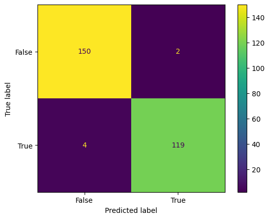
y_pred_bill = tree_classifier.predict(X_test_bill)

conf_mtx_bill = confusion_matrix(y_test_bill, y_pred_bill)
conf_mtx_bill

# array([[150,   2],
#        [  4, 119]])

conf_mtx_bill_plot = ConfusionMatrixDisplay(
    confusion_matrix=conf_mtx_bill,
    display_labels=[False,True]
)

conf_mtx_bill_plot.plot()
plt.show()

report_bill = classification_report(
    y_test_bill, y_pred_bill
)
print(report_bill)

	precision	recall	f1-score	support
0	0.97	0.99	0.98	152
1	0.98	0.97	0.98	123
accuracy			0.98	275
macro avg	0.98	0.98	0.98	275
weighted avg	0.98	0.98	0.98	275

Supervised Learning - Random Forest Classifier

• Does not require normalization
• Is not sensitive to missing values
• Low risk of overfitting
• Efficient with large datasets
• High accuracy

Dataset

!wget https://raw.githubusercontent.com/xjcjiacheng/data-analysis/master/heart%20disease%20UCI/heart.csv -P datasets

heart_df = pd.read_csv('datasets/heart.csv')
heart_df.head(5)

	age	sex	cp	trestbps	chol	fbs	restecg	thalach	exang	oldpeak	slope	ca	thal	target
0	63	1	3	145	233	1	0	150	0	2.3	0	0	1	1
1	37	1	2	130	250	0	1	187	0	3.5	0	0	2	1
2	41	0	1	130	204	0	0	172	0	1.4	2	0	2	1
3	56	1	1	120	236	0	1	178	0	0.8	2	0	2	1
4	57	0	0	120	354	0	1	163	1	0.6	2	0	2	1

Preprocessing

# remove target feature from training set
X_heart = heart_df.drop('target', axis=1)
y_heart = heart_df['target']

X_train_heart, X_test_heart, y_train_heart, y_test_heart = train_test_split(
    X_heart,
    y_heart,
    test_size=0.2,
    random_state=0
)

Model Fitting

forest_classifier = RandomForestClassifier(n_estimators=10, criterion='entropy')

forest_classifier.fit(X_train_heart, y_train_heart)

Evaluation

y_pred_heart = forest_classifier.predict(X_test_heart)

conf_mtx_heart = confusion_matrix(y_test_heart, y_pred_heart)
conf_mtx_heart

# array([[24,  3],
#        [ 5, 29]])

conf_mtx_heart_plot = ConfusionMatrixDisplay(
    confusion_matrix=conf_mtx_heart,
    display_labels=[False,True]
)

conf_mtx_heart_plot.plot()
plt.show()

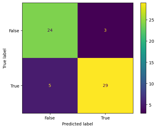
report_heart = classification_report(
    y_test_heart, y_pred_heart
)
print(report_heart)

	precision	recall	f1-score	support
0	0.83	0.89	0.86	27
1	0.91	0.85	0.88	34
accuracy			0.87	61
macro avg	0.87	0.87	0.87	61
weighted avg	0.87	0.87	0.87	61

Random Forest Hyperparameter Tuning

Testing Hyperparameters

rdnfor_classifier = RandomForestClassifier(
    n_estimators=2,
    min_samples_split=2,
    min_samples_leaf=1,
    criterion='entropy'
)
rdnfor_classifier.fit(X_train_heart, y_train_heart)

rdnfor_pred = rdnfor_classifier.predict(X_test_heart)
print('Accuracy Score: ', accuracy_score(y_test_heart, rdnfor_pred).round(4)*100, '%')

# Accuracy Score:  73.77 %

Grid-Search Cross-Validation

Try a set of values for selected Hyperparameter to find the optimal configuration.

param_grid = \{
    'n_estimators': [5, 25, 50, 75,100, 125],
    'min_samples_split': [1,2,3],
    'min_samples_leaf': [1,2,3],
    'criterion': ['gini', 'entropy', 'log_loss'],
    'max_features' : ['sqrt', 'log2']
\}

grid_search = GridSearchCV(
    estimator = rdnfor_classifier,
    param_grid = param_grid
)

grid_search.fit(X_train_heart, y_train_heart)

print('Best Parameter: ', grid_search.best_params_)
# Best Parameter:  \{
# 'criterion': 'entropy',
# 'max_features': 'sqrt',
# 'min_samples_leaf': 2,
# 'min_samples_split': 1,
# 'n_estimators': 25
# \}

rdnfor_classifier_optimized = RandomForestClassifier(
    n_estimators=25,
    min_samples_split=1,
    min_samples_leaf=2,
    criterion='entropy',
    max_features='sqrt'
)

rdnfor_classifier_optimized.fit(X_train_heart, y_train_heart)

rdnfor_pred_optimized = rdnfor_classifier_optimized.predict(X_test_heart)
print('Accuracy Score: ', accuracy_score(y_test_heart, rdnfor_pred_optimized).round(4)*100, '%')

# Accuracy Score:  85.25 %

Random Forest Classifier 1 - Penguins

!wget https://github.com/remijul/dataset/raw/master/penguins_size.csv -P datasets

peng_df = pd.read_csv('datasets/penguins_size.csv')
peng_df = peng_df.dropna()
peng_df.head(5)

	species	island	culmen_length_mm	culmen_depth_mm	flipper_length_mm	body_mass_g	sex
0	Adelie	Torgersen	39.1	18.7	181.0	3750.0	MALE
1	Adelie	Torgersen	39.5	17.4	186.0	3800.0	FEMALE
2	Adelie	Torgersen	40.3	18.0	195.0	3250.0	FEMALE
4	Adelie	Torgersen	36.7	19.3	193.0	3450.0	FEMALE
5	Adelie	Torgersen	39.3	20.6	190.0	3650.0	MALE

# drop labels and encode string values
X_peng = pd.get_dummies(peng_df.drop('species', axis=1),drop_first=True)
y_peng = peng_df['species']

# train/test split
X_peng_train, X_peng_test, y_peng_train, y_peng_test = train_test_split(
    X_peng,
    y_peng,
    test_size=0.3,
    random_state=42
)

# creating the model
rfc_peng = RandomForestClassifier(
    n_estimators=10,
    max_features='sqrt',
    random_state=42
)

# model training and running predictions
rfc_peng.fit(X_peng_train, y_peng_train)
peng_pred = rfc_peng.predict(X_peng_test)
print('Accuracy Score: ',accuracy_score(y_peng_test, peng_pred, normalize=True).round(4)*100, '%')
# Accuracy Score:  98.02 %

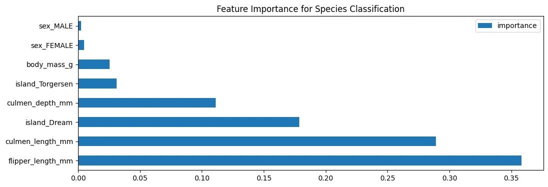
Feature Importance

# feature importance for classification
peng_index = ['importance']
peng_data_columns = pd.Series(X_peng.columns)
peng_importance_array = rfc_peng.feature_importances_
peng_importance_df = pd.DataFrame(peng_importance_array, peng_data_columns, peng_index)
peng_importance_df

	importance
culmen_length_mm	0.288928
culmen_depth_mm	0.111021
flipper_length_mm	0.357994
body_mass_g	0.025477
island_Dream	0.178498
island_Torgersen	0.031042
sex_FEMALE	0.004716
sex_MALE	0.002324

peng_importance_df.sort_values(
    by='importance',
    ascending=False
).plot(
    kind='barh',
    title='Feature Importance for Species Classification',
    figsize=(12,4)
)

Model Evaluation

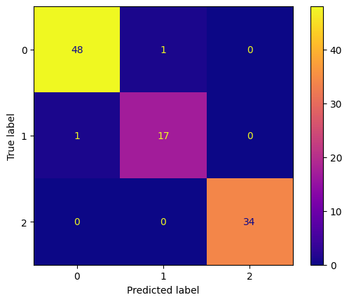
report_peng = classification_report(y_peng_test, peng_pred)
print(report_peng)

	precision	recall	f1-score	support
Adelie	0.98	0.98	0.98	49
Chinstrap	0.94	0.94	0.94	18
Gentoo	1.00	1.00	1.00	34
accuracy			0.98	101
macro avg	0.97	0.97	0.97	101
weighted avg	0.98	0.98	0.98	101

conf_mtx_peng = confusion_matrix(y_peng_test, peng_pred)

conf_mtx_peng_plot = ConfusionMatrixDisplay(
    confusion_matrix=conf_mtx_peng
)

conf_mtx_peng_plot.plot(cmap='plasma')

Random Forest Classifier - Banknote Authentication

!wget https://github.com/jbrownlee/Datasets/raw/master/banknote_authentication.csv -P datasets

money_df = pd.read_csv('datasets/data-banknote-authentication.csv')
money_df.head(5)

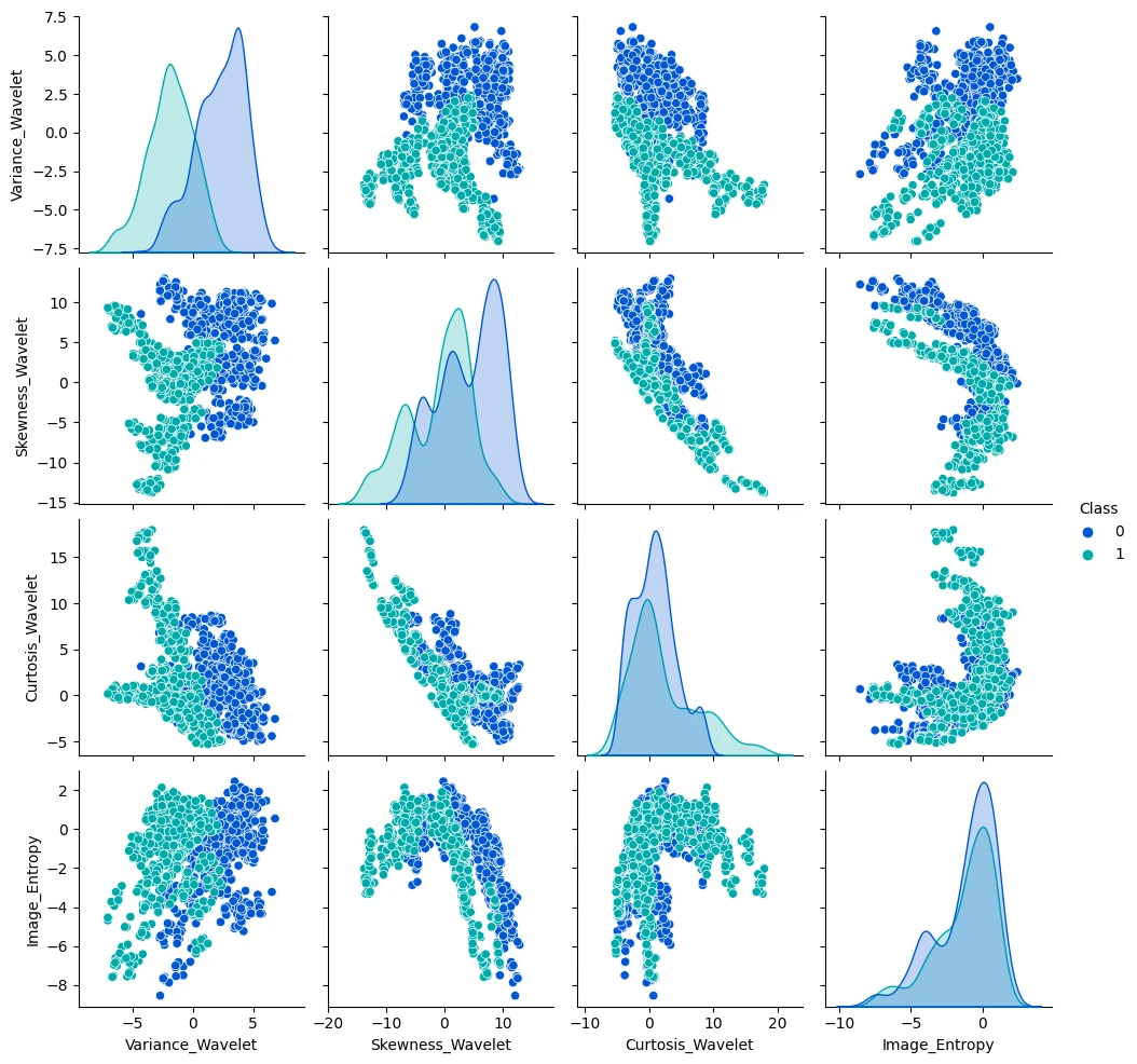
	Variance_Wavelet	Skewness_Wavelet	Curtosis_Wavelet	Image_Entropy	Class
0	3.62160	8.6661	-2.8073	-0.44699	0
1	4.54590	8.1674	-2.4586	-1.46210	0
2	3.86600	-2.6383	1.9242	0.10645	0
3	3.45660	9.5228	-4.0112	-3.59440	0
4	0.32924	-4.4552	4.5718	-0.98880	0

sns.pairplot(money_df, hue='Class', palette='winter')

# drop label for training
X_money = money_df.drop('Class', axis=1)
y_money = money_df['Class']
print(X_money.shape, y_money.shape)

X_money_train, X_money_test, y_money_train, y_money_test = train_test_split(
    X_money,
    y_money,
    test_size=0.15,
    random_state=42
)

Grid Search for Hyperparameters

rfc_money_base = RandomForestClassifier(oob_score=True)

param_grid = \{
    'n_estimators': [64, 96, 128, 160, 192],
    'max_features': [2,3,4],
    'bootstrap': [True, False]
\}

grid_money = GridSearchCV(rfc_money_base, param_grid) 
grid_money.fit(X_money_train, y_money_train)
grid_money.best_params_
# \{'bootstrap': True, 'max_features': 2, 'n_estimators': 96\}

Model Training and Evaluation

rfc_money = RandomForestClassifier(
    bootstrap=True,
    max_features=2,
    n_estimators=96,
    oob_score=True
)
rfc_money.fit(X_money_train, y_money_train)
print('Out-of-Bag Score: ', rfc_money.oob_score_.round(4)*100, '%')
# Out-of-Bag Score:  99.14 %

money_pred = rfc_money.predict(X_money_test)
money_report = classification_report(y_money_test, money_pred)
print(money_report)

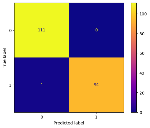
	precision	recall	f1-score	support
0	0.99	1.00	1.00	111
1	1.00	0.99	0.99	95
accuracy			1.00	206
macro avg	1.00	0.99	1.00	206
weighted avg	1.00	1.00	1.00	206

conf_mtx_money = confusion_matrix(y_money_test, money_pred)

conf_mtx_money_plot = ConfusionMatrixDisplay(
    confusion_matrix=conf_mtx_money
)

conf_mtx_money_plot.plot(cmap='plasma')

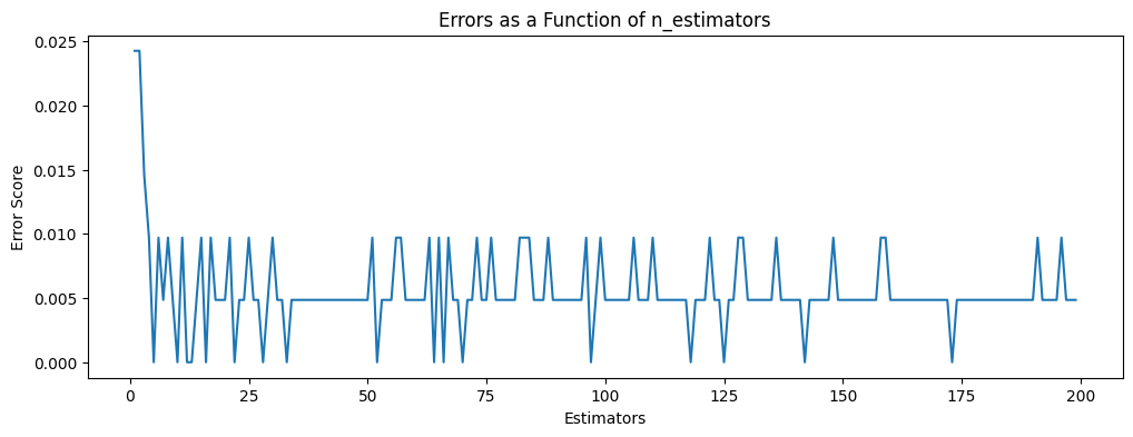
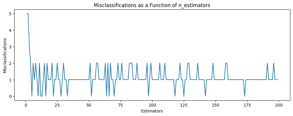
Optimizations

# verify number of estimators found by grid search
errors = []
missclassifications = []

for n in range(1,200):
    rfc = RandomForestClassifier(n_estimators=n, max_features=2)
    rfc.fit(X_money_train, y_money_train)
    preds = rfc.predict(X_money_test)
    
    err = 1 - accuracy_score(y_money_test, preds)
    errors.append(err)
    
    n_missed = np.sum(preds != y_money_test)
    missclassifications.append(n_missed)

plt.figure(figsize=(12,4))
plt.title('Errors as a Function of n_estimators')
plt.xlabel('Estimators')
plt.ylabel('Error Score')
plt.plot(range(1,200), errors)
# there is no noteable improvement above ~10 estimators

plt.figure(figsize=(12,4))
plt.title('Misclassifications as a Function of n_estimators')
plt.xlabel('Estimators')
plt.ylabel('Misclassifications')
plt.plot(range(1,200), missclassifications)
# and the same for misclassifications

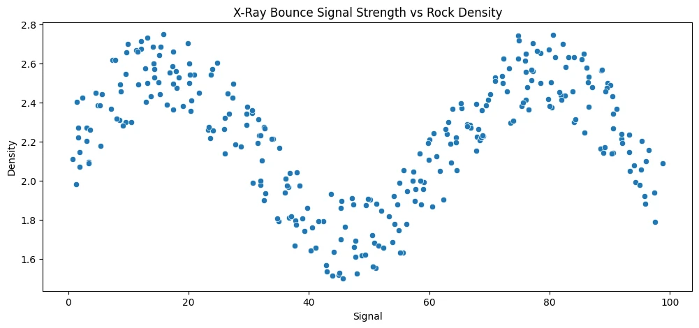
Random Forest Regressor

Comparing different regression models to a random forrest regression model.

# dataset
!wget https://github.com/vineetsingh028/Rock_Density_Prediction/raw/master/rock_density_xray.csv -P datasets

rock_df = pd.read_csv('datasets/rock_density_xray.csv')
rock_df.columns = ['Signal', 'Density']
rock_df.head(5)

	Signal	Density
0	72.945124	2.456548
1	14.229877	2.601719
2	36.597334	1.967004
3	9.578899	2.300439
4	21.765897	2.452374

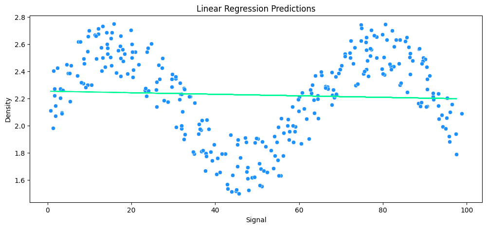
plt.figure(figsize=(12,5))
plt.title('X-Ray Bounce Signal Strength vs Rock Density')
sns.scatterplot(data=rock_df, x='Signal', y='Density')
# the signal vs density plot follows a sine wave - spoiler alert: simpler algorithm
# will fail trying to fit this dataset...

# train-test split
X_rock = rock_df['Signal'].values.reshape(-1,1)
y_rock = rock_df['Density']

X_rock_train, X_rock_test, y_rock_train, y_rock_test = train_test_split(
    X_rock,
    y_rock,
    test_size=0.1,
    random_state=42
)

# normalization
scaler = StandardScaler()
X_rock_train_scaled = scaler.fit_transform(X_rock_train)
X_rock_test_scaled = scaler.transform(X_rock_test)

vs Linear Regression

lr_rock = LinearRegression()
lr_rock.fit(X_rock_train_scaled, y_rock_train)

lr_rock_preds = lr_rock.predict(X_rock_test_scaled)

mae = mean_absolute_error(y_rock_test, lr_rock_preds)
rmse = np.sqrt(mean_squared_error(y_rock_test, lr_rock_preds))
mean_abs = y_rock_test.mean()
avg_error = mae * 100 / mean_abs

print('MAE: ', mae.round(2), 'RMSE: ', rmse.round(2), 'Relative Avg. Error: ', avg_error.round(2), '%')
# MAE:  0.24 RMSE:  0.3 Relative Avg. Error:  10.93 %

# visualize predictions
plt.figure(figsize=(12,5))
plt.plot(X_rock_test, lr_rock_preds, c='mediumspringgreen')
sns.scatterplot(data=rock_df, x='Signal', y='Density', c='dodgerblue')
plt.title('Linear Regression Predictions')
plt.show()
# the returned error appears small because the linear regression returns an average
# but it cannot fit a linear line to the contours of the underlying sine wave function

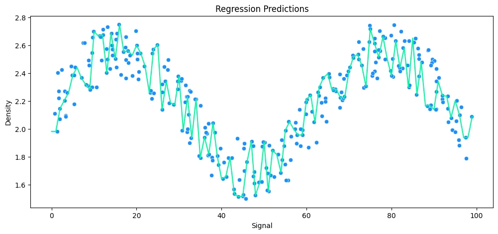
vs Polynomial Regression

# helper function
def run_model(model, X_train, y_train, X_test, y_test, df):
    
    # FIT MODEL
    model.fit(X_train, y_train)
    
    # EVALUATE
    y_preds = model.predict(X_test)
    mae = mean_absolute_error(y_test, y_preds)
    rmse = np.sqrt(mean_squared_error(y_test, y_preds))
    mean_abs = y_test.mean()
    avg_error = mae * 100 / mean_abs
    print('MAE: ', mae.round(2), 'RMSE: ', rmse.round(2), 'Relative Avg. Error: ', avg_error.round(2), '%')
    
    # PLOT RESULTS
    signal_range = np.arange(0,100)
    output = model.predict(signal_range.reshape(-1,1))
    
    
    plt.figure(figsize=(12,5))
    sns.scatterplot(data=df, x='Signal', y='Density', c='dodgerblue')
    plt.plot(signal_range,output, c='mediumspringgreen')
    plt.title('Regression Predictions')
    plt.show()

# test helper on previous linear regression
run_model(
    model=lr_rock,
    X_train=X_rock_train,
    y_train=y_rock_train,
    X_test=X_rock_test,
    y_test=y_rock_test,
    df=rock_df
)

MAE: 0.24 RMSE: 0.3 Relative Avg. Error: 10.93 %

# build polynomial model
pipe_poly = make_pipeline(
    PolynomialFeatures(degree=6),
    LinearRegression()
)

# run model
run_model(
    model=pipe_poly,
    X_train=X_rock_train,
    y_train=y_rock_train,
    X_test=X_rock_test,
    y_test=y_rock_test,
    df=rock_df
)
# with a HARD LIMIT of 0-100 for the xray signal a 6th degree polinomial is a good fit

MAE: 0.13 RMSE: 0.14 Relative Avg. Error: 5.7 %

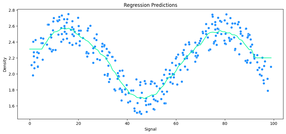
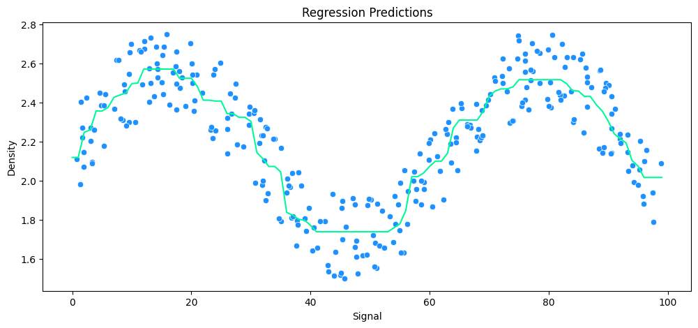
vs KNeighbors Regression

# build polynomial model
k_values=[1,5,10,25]

for k in k_values:
    model = KNeighborsRegressor(n_neighbors=k)
    print(model)
    
    # run model
    run_model(
        model,
        X_train=X_rock_train,
        y_train=y_rock_train,
        X_test=X_rock_test,
        y_test=y_rock_test,
        df=rock_df
    )

KNeighborsRegressor(n_neighbors=1)

MAE: 0.12 RMSE: 0.17 Relative Avg. Error: 5.47 %

KNeighborsRegressor()

MAE: 0.13 RMSE: 0.15 Relative Avg. Error: 5.9 %

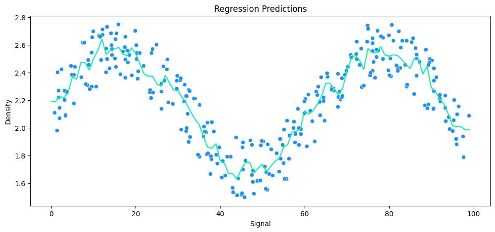
KNeighborsRegressor(n_neighbors=10)

MAE: 0.12 RMSE: 0.14 Relative Avg. Error: 5.44 %

KNeighborsRegressor(n_neighbors=25)

MAE: 0.14 RMSE: 0.16 Relative Avg. Error: 6.18 %

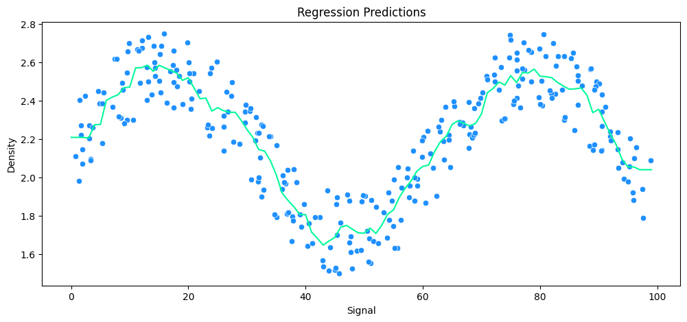
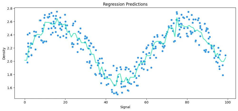
vs Decision Tree Regression

tree_model = DecisionTreeRegressor()

# run model
run_model(
    model=tree_model,
    X_train=X_rock_train,
    y_train=y_rock_train,
    X_test=X_rock_test,
    y_test=y_rock_test,
    df=rock_df
)

MAE: 0.12 RMSE: 0.17 Relative Avg. Error: 5.47 %

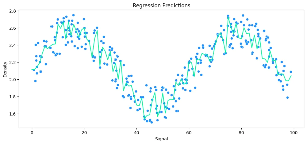
vs Support Vector Regression

svr_rock = svm.SVR()

param_grid = \{
    'C': [0.01,0.1,1,5,10,100, 1000],
    'gamma': ['auto', 'scale']
\}

rock_grid = GridSearchCV(svr_rock, param_grid)

# run model
run_model(
    model=rock_grid,
    X_train=X_rock_train,
    y_train=y_rock_train,
    X_test=X_rock_test,
    y_test=y_rock_test,
    df=rock_df
)

MAE: 0.13 RMSE: 0.14 Relative Avg. Error: 5.75 %

vs Gradient Boosting Regression

gbr_rock = GradientBoostingRegressor()

# run model
run_model(
    model=gbr_rock,
    X_train=X_rock_train,
    y_train=y_rock_train,
    X_test=X_rock_test,
    y_test=y_rock_test,
    df=rock_df
)

MAE: 0.13 RMSE: 0.15 Relative Avg. Error: 5.76 %

vs Ada Boosting Regression

abr_rock = AdaBoostRegressor()

# run model
run_model(
    model=abr_rock,
    X_train=X_rock_train,
    y_train=y_rock_train,
    X_test=X_rock_test,
    y_test=y_rock_test,
    df=rock_df
)

MAE: 0.13 RMSE: 0.14 Relative Avg. Error: 5.67 %

Finally, Random Forrest Regression

rfr_rock = RandomForestRegressor(n_estimators=10)

# run model
run_model(
    model=rfr_rock,
    X_train=X_rock_train,
    y_train=y_rock_train,
    X_test=X_rock_test,
    y_test=y_rock_test,
    df=rock_df
)

MAE: 0.11 RMSE: 0.14 Relative Avg. Error: 5.1 %

Supervised Learning - SVC Model

Support Vector Machines (SVMs) are a set of supervised learning methods used for classification, regression and outliers detection.

• Effective in high dimensional spaces.
• Still effective in cases where number of dimensions is greater than the number of samples.

Dataset

• Three different varieties of the wheat - Kaggle.com

Measurements of geometrical properties of kernels belonging to three different varieties of wheat:

• A: Area,
• P: Perimeter,
• C = 4piA/P^2: Compactness,
• LK: Length of kernel,
• WK: Width of kernel,
• A_Coef: Asymmetry coefficient
• LKG: Length of kernel groove.

!wget https://raw.githubusercontent.com/prasertcbs/basic-dataset/master/Seed_Data.csv -P datasets

wheat_df = pd.read_csv('datasets/Seed_Data.csv')
wheat_df.head(5)

	A	P	C	LK	WK	A_Coef	LKG	target
0	15.26	14.84	0.8710	5.763	3.312	2.221	5.220	0
1	14.88	14.57	0.8811	5.554	3.333	1.018	4.956	0
2	14.29	14.09	0.9050	5.291	3.337	2.699	4.825	0
3	13.84	13.94	0.8955	5.324	3.379	2.259	4.805	0
4	16.14	14.99	0.9034	5.658	3.562	1.355	5.175	0

wheat_df.info()

# <class 'pandas.core.frame.DataFrame'>
# RangeIndex: 210 entries, 0 to 209
# Data columns (total 8 columns):
#  #   Column  Non-Null Count  Dtype  
# ---  ------  --------------  -----  
#  0   A       210 non-null    float64
#  1   P       210 non-null    float64
#  2   C       210 non-null    float64
#  3   LK      210 non-null    float64
#  4   WK      210 non-null    float64
#  5   A_Coef  210 non-null    float64
#  6   LKG     210 non-null    float64
#  7   target  210 non-null    int64  
# dtypes: float64(7), int64(1)
# memory usage: 13.2 KB

Preprocessing

# remove target feature from training set
X_wheat = wheat_df.drop('target', axis=1)
y_wheat = wheat_df['target']

print(X_wheat.shape, y_wheat.shape)
# (210, 7) (210,)

# train/test split
X_train_wheat, X_test_wheat, y_train_wheat, y_test_wheat = train_test_split(
    X_wheat,
    y_wheat,
    test_size=0.2,
    random_state=42
)

# normalization
sc_wheat = StandardScaler()
X_train_wheat=sc_wheat.fit_transform(X_train_wheat)
X_test_wheat=sc_wheat.fit_transform(X_test_wheat)

Model Training

# SVM classifier fitting
clf_wheat = svm.SVC()
clf_wheat.fit(X_train_wheat, y_train_wheat)

Model Evaluation

# Predictions
y_wheat_pred = clf_wheat.predict(X_test_wheat)

print(
    'Accuracy Score: ',
    accuracy_score(y_test_wheat, y_wheat_pred, normalize=True).round(4)*100, '%'
)
# Accuracy Score:  90.48 %

report_wheat = classification_report(
    y_test_wheat, y_wheat_pred
)
print(report_wheat)

	precision	recall	f1-score	support
0	0.82	0.82	0.82	11
1	1.00	0.93	0.96	14
2	0.89	0.94	0.91	17
accuracy			0.90	42
macro avg	0.90	0.90	0.90	42
weighted avg	0.91	0.90	0.91	42

conf_mtx_wheat = confusion_matrix(y_test_wheat, y_wheat_pred)
conf_mtx_wheat

# array([[ 9,  0,  2],
#        [ 1, 13,  0],
#        [ 1,  0, 16]])

conf_mtx_wheat_plot = ConfusionMatrixDisplay(
    confusion_matrix=conf_mtx_wheat
)

conf_mtx_wheat_plot.plot()
plt.show()

Margin Plots for Support Vector Classifier

# get dataset
!wget https://github.com/alpeshraj/mouse_viral_study/raw/main/mouse_viral_study.csv -P datasets

mice_df = pd.read_csv('datasets/mouse_viral_study.csv')
mice_df.head(5)

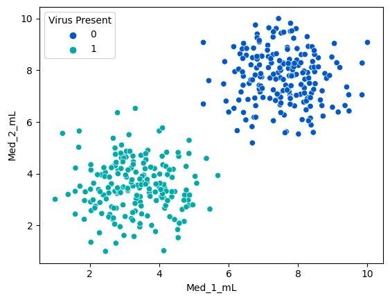
	Med_1_mL	Med_2_mL	Virus Present
0	6.508231	8.582531	0
1	4.126116	3.073459	1
2	6.427870	6.369758	0
3	3.672953	4.905215	1
4	1.580321	2.440562	1

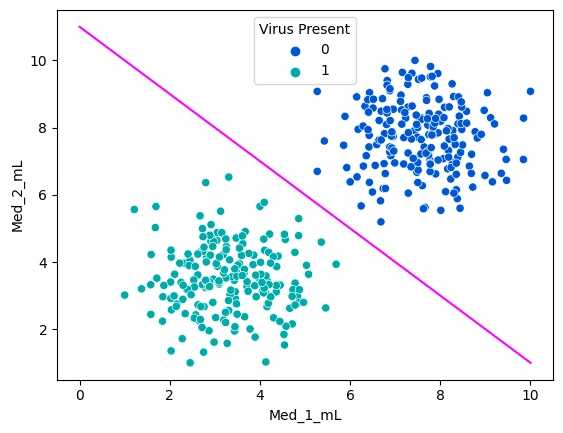
sns.scatterplot(data=mice_df, x='Med_1_mL',y='Med_2_mL',hue='Virus Present', palette='winter')

# visualizing a hyperplane to separate the two features
sns.scatterplot(data=mice_df, x='Med_1_mL',y='Med_2_mL',hue='Virus Present', palette='winter')

x = np.linspace(0,10,100)
m = -1
b = 11
y = m*x + b

plt.plot(x,y,c='fuchsia')

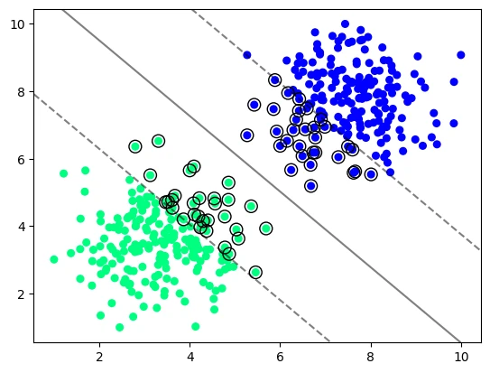
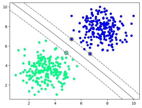
SVC with a Linear Kernel

# using a support vector classifier to calculate maximize the margin between both classes

y_vir = mice_df['Virus Present']
X_vir = mice_df.drop('Virus Present',axis=1)

# kernel : \{'linear', 'poly', 'rbf', 'sigmoid', 'precomputed'\}
# the smaller the C value the more feature vectors will be inside the margin
model_vir = svm.SVC(kernel='linear', C=1000)

model_vir.fit(X_vir, y_vir)

# import helper function
from helper.svm_margin_plot import plot_svm_boundary

plot_svm_boundary(model_vir, X_vir, y_vir)

# the smaller the C value the more feature vectors will be inside the margin
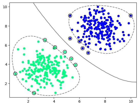
model_vir_low_reg = svm.SVC(kernel='linear', C=0.005)
model_vir_low_reg.fit(X_vir, y_vir)
plot_svm_boundary(model_vir_low_reg, X_vir, y_vir)

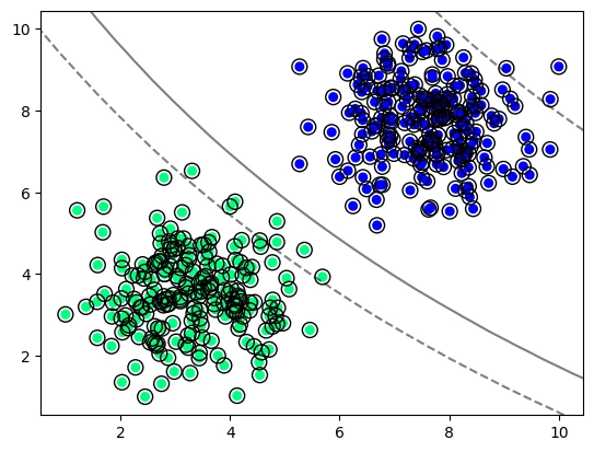
SVC with a Radial Basis Function Kernel

model_vir_rbf = svm.SVC(kernel='rbf', C=1)
model_vir_rbf.fit(X_vir, y_vir)
plot_svm_boundary(model_vir_rbf, X_vir, y_vir)

# # gamma : \{'scale', 'auto'\} or float, default='scale'
# - if ``gamma='scale'`` (default) is passed then it uses 1 / (n_features * X.var()) as value of gamma,
# - if 'auto', uses 1 / n_features
# - if float, must be non-negative.
model_vir_rbf_auto_gamma = svm.SVC(kernel='rbf', C=1, gamma='auto')
model_vir_rbf_auto_gamma.fit(X_vir, y_vir)
plot_svm_boundary(model_vir_rbf_auto_gamma, X_vir, y_vir)

SVC with a Sigmoid Kernel

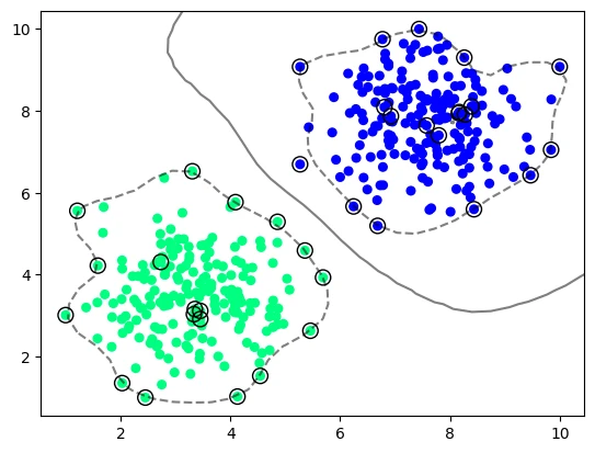
model_vir_sigmoid = svm.SVC(kernel='sigmoid', gamma='scale')
model_vir_sigmoid.fit(X_vir, y_vir)
plot_svm_boundary(model_vir_sigmoid, X_vir, y_vir)

SVC with a Polynomial Kernel

model_vir_poly = svm.SVC(kernel='poly', C=1, degree=2)
model_vir_poly.fit(X_vir, y_vir)
plot_svm_boundary(model_vir_poly, X_vir, y_vir)

Grid Search for Support Vector Classifier

svm_base_model = svm.SVC()

param_grid = \{
    'C':[0.01, 0.1, 1],
    'kernel': ['linear', 'rbf']
\}

grid = GridSearchCV(svm_base_model, param_grid) 
grid.fit(X_vir, y_vir)

grid.best_params_
# \{'C': 0.01, 'kernel': 'linear'\}

Support Vector Regression

# dataset
!wget https://github.com/fsdhakan/ML/raw/main/cement_slump.csv -P datasets

cement_df = pd.read_csv('datasets/cement_slump.csv')
cement_df.head(5)

	Cement	Slag	Fly ash	Water	SP	Coarse Aggr.	Fine Aggr.	SLUMP(cm)	FLOW(cm)	Compressive Strength (28-day)(Mpa)
0	273.0	82.0	105.0	210.0	9.0	904.0	680.0	23.0	62.0	34.99
1	163.0	149.0	191.0	180.0	12.0	843.0	746.0	0.0	20.0	41.14
2	162.0	148.0	191.0	179.0	16.0	840.0	743.0	1.0	20.0	41.81
3	162.0	148.0	190.0	179.0	19.0	838.0	741.0	3.0	21.5	42.08
4	154.0	112.0	144.0	220.0	10.0	923.0	658.0	20.0	64.0	26.82

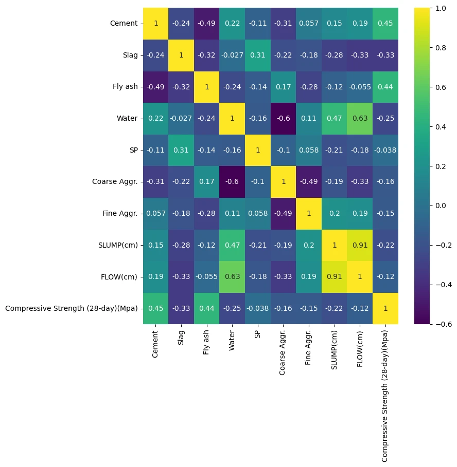
plt.figure(figsize=(8,8))
sns.heatmap(cement_df.corr(), annot=True, cmap='viridis')

# drop labels
X_cement = cement_df.drop('Compressive Strength (28-day)(Mpa)', axis=1)
y_cement = cement_df['Compressive Strength (28-day)(Mpa)']

 # train/test split
    X_train_cement, X_test_cement, y_train_cement, y_test_cement = train_test_split(
     X_cement,
     y_cement,
     test_size=0.3,
     random_state=42
 )

# normalize
scaler = StandardScaler()
X_train_cement_scaled = scaler.fit_transform(X_train_cement)
X_test_cement_scaled = scaler.transform(X_test_cement)

Base Model Run

base_model_cement = svm.SVR()

base_model_cement.fit(X_train_cement_scaled, y_train_cement)

base_model_predictions = base_model_cement.predict(X_test_cement_scaled)

mae = mean_absolute_error(y_test_cement, base_model_predictions)
rmse = mean_squared_error(y_test_cement, base_model_predictions)
mean_abs = y_test_cement.mean()
avg_error = mae * 100 / mean_abs

print('MAE: ', mae.round(2), 'RMSE: ', rmse.round(2), 'Relative Avg. Error: ', avg_error.round(2), '%')

MAE	RMSE	Relative Avg. Error
4.68	36.95	12.75 %

Grid Search for better Hyperparameter

param_grid = \{
    'C': [0.001,0.01,0.1,0.5,1],
    'kernel': ['linear', 'rbf', 'poly'],
    'gamma': ['scale', 'auto'],
    'degree': [2,3,4],
    'epsilon': [0,0.01,0.1,0.5,1,2]
\}

cement_grid = GridSearchCV(base_model_cement, param_grid)
cement_grid.fit(X_train_cement_scaled, y_train_cement)

cement_grid.best_params_
# \{'C': 1, 'degree': 2, 'epsilon': 2, 'gamma': 'scale', 'kernel': 'linear'\}

cement_grid_predictions = cement_grid.predict(X_test_cement_scaled)

mae_grid = mean_absolute_error(y_test_cement, cement_grid_predictions)
rmse_grid = mean_squared_error(y_test_cement, cement_grid_predictions)
mean_abs = y_test_cement.mean()
avg_error_grid = mae_grid * 100 / mean_abs

print('MAE: ', mae_grid.round(2), 'RMSE: ', rmse_grid.round(2), 'Relative Avg. Error: ', avg_error_grid.round(2), '%')

MAE	RMSE	Relative Avg. Error
1.85	5.2	5.05 %

Example Task - Wine Fraud

Data Exploration

# dataset
!wget https://github.com/CAPGAGA/Fraud-in-Wine/raw/main/wine_fraud.csv -P datasets

wine_df = pd.read_csv('datasets/wine_fraud.csv')
wine_df.head(5)

	fixed acidity	volatile acidity	citric acid	residual sugar	chlorides	free sulfur dioxide	total sulfur dioxide	density	pH	sulphates	alcohol	quality	type
0	7.4	0.70	0.00	1.9	0.076	11.0	34.0	0.9978	3.51	0.56	9.4	Legit	red
1	7.8	0.88	0.00	2.6	0.098	25.0	67.0	0.9968	3.20	0.68	9.8	Legit	red
2	7.8	0.76	0.04	2.3	0.092	15.0	54.0	0.9970	3.26	0.65	9.8	Legit	red
3	11.2	0.28	0.56	1.9	0.075	17.0	60.0	0.9980	3.16	0.58	9.8	Legit	red
4	7.4	0.70	0.00	1.9	0.076	11.0	34.0	0.9978	3.51	0.56	9.4	Legit	red

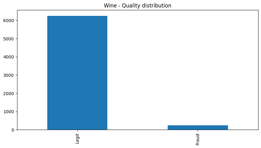
wine_df.value_counts('quality')

quality
Legit	6251
Fraud	246
dtype: int64

wine_df['quality'].value_counts().plot(
    kind='bar',
    figsize=(10,5), 
    title='Wine - Quality distribution')

plt.figure(figsize=(10, 5))
plt.title('Wine - Quality distribution by Type')

sns.countplot(
    data=wine_df,
    x='quality',
    hue='type',
    palette='winter'
)

plt.savefig('assets/Scikit_Learn_22.webp', bbox_inches='tight')

wine_df_white = wine_df[wine_df['type'] == 'white']
wine_df_red = wine_df[wine_df['type'] == 'red']

# fraud percentage by wine type
legit_white_wines = wine_df_white.value_counts('quality')[0]
fraud_white_wines = wine_df_white.value_counts('quality')[1]
white_fraud_percentage = fraud_white_wines * 100 / (legit_white_wines + fraud_white_wines)

legit_red_wines = wine_df_red.value_counts('quality')[0]
fraud_red_wines = wine_df_red.value_counts('quality')[1]
red_fraud_percentage = fraud_red_wines * 100 / (legit_red_wines + fraud_red_wines)

print(
    'Fraud Percentage: \nWhite Wines: ',
    white_fraud_percentage.round(2),
    '% \nRed Wines: ',
    red_fraud_percentage.round(2),
    '%'
)

Fraud Percentage:
White Wines:	3.74 %
Red Wines:	3.94 %

# make features numeric
feature_map = \{
    'Legit': 0,
    'Fraud': 1,
    'red': 0,
    'white': 1
\}

wine_df['quality_enc'] = wine_df['quality'].map(feature_map)
wine_df['type_enc'] = wine_df['type'].map(feature_map)
wine_df[['quality', 'quality_enc', 'type', 'type_enc']]

	quality	quality_enc	type	type_enc
0	Legit	0	red	0
1	Legit	0	red	0
2	Legit	0	red	0
3	Legit	0	red	0
4	Legit	0	red	0
...
6492	Legit	0	white	1
6493	Legit	0	white	1
6494	Legit	0	white	1
6495	Legit	0	white	1
6496	Legit	0	white	1
6497 rows × 4 columns

# find correlations
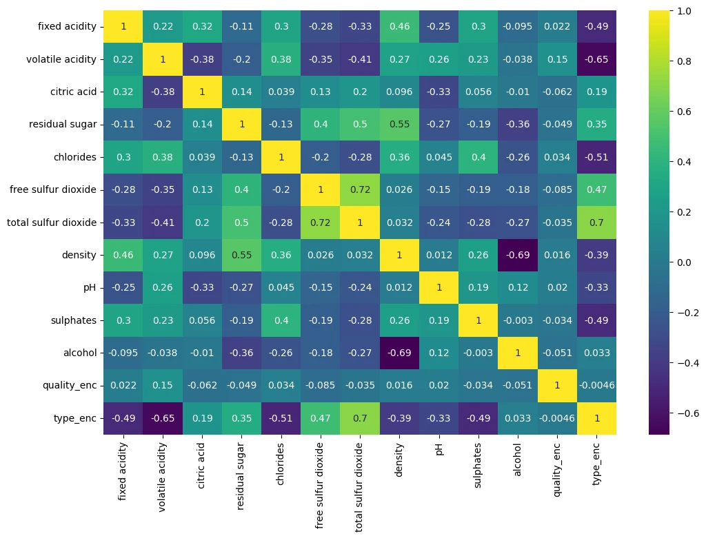
wine_df.corr(numeric_only=True)

	fixed acidity	volatile acidity	citric acid	residual sugar	chlorides	free sulfur dioxide	total sulfur dioxide	density	pH	sulphates	alcohol	quality_enc	type_enc
fixed acidity	1.000000	0.219008	0.324436	-0.111981	0.298195	-0.282735	-0.329054	0.458910	-0.252700	0.299568	-0.095452	0.021794	-0.486740
volatile acidity	0.219008	1.000000	-0.377981	-0.196011	0.377124	-0.352557	-0.414476	0.271296	0.261454	0.225984	-0.037640	0.151228	-0.653036
citric acid	0.324436	-0.377981	1.000000	0.142451	0.038998	0.133126	0.195242	0.096154	-0.329808	0.056197	-0.010493	-0.061789	0.187397
residual sugar	-0.111981	-0.196011	0.142451	1.000000	-0.128940	0.402871	0.495482	0.552517	-0.267320	-0.185927	-0.359415	-0.048756	0.348821
chlorides	0.298195	0.377124	0.038998	-0.128940	1.000000	-0.195045	-0.279630	0.362615	0.044708	0.395593	-0.256916	0.034499	-0.512678
free sulfur dioxide	-0.282735	-0.352557	0.133126	0.402871	-0.195045	1.000000	0.720934	0.025717	-0.145854	-0.188457	-0.179838	-0.085204	0.471644
total sulfur dioxide	-0.329054	-0.414476	0.195242	0.495482	-0.279630	0.720934	1.000000	0.032395	-0.238413	-0.275727	-0.265740	-0.035252	0.700357
density	0.458910	0.271296	0.096154	0.552517	0.362615	0.025717	0.032395	1.000000	0.011686	0.259478	-0.686745	0.016351	-0.390645
pH	-0.252700	0.261454	-0.329808	-0.267320	0.044708	-0.145854	-0.238413	0.011686	1.000000	0.192123	0.121248	0.020107	-0.329129
sulphates	0.299568	0.225984	0.056197	-0.185927	0.395593	-0.188457	-0.275727	0.259478	0.192123	1.000000	-0.003029	-0.034046	-0.487218
alcohol	-0.095452	-0.037640	-0.010493	-0.359415	-0.256916	-0.179838	-0.265740	-0.686745	0.121248	-0.003029	1.000000	-0.051141	0.032970
quality_enc	0.021794	0.151228	-0.061789	-0.048756	0.034499	-0.085204	-0.035252	0.016351	0.020107	-0.034046	-0.051141	1.000000	-0.004598
type_enc	-0.486740	-0.653036	0.187397	0.348821	-0.512678	0.471644	0.700357	-0.390645	-0.329129	-0.487218	0.032970	-0.004598	1.000000

plt.figure(figsize=(12,8))
sns.heatmap(wine_df.corr(numeric_only=True), annot=True, cmap='viridis')

# how does the quality correlate to measurements
wine_df.corr(numeric_only=True)['quality_enc']

Quality Correlstion
fixed acidity	0.021794
volatile acidity	0.151228
citric acid	-0.061789
residual sugar	-0.048756
chlorides	0.034499
free sulfur dioxide	-0.085204
total sulfur dioxide	-0.035252
density	0.016351
pH	0.020107
sulphates	-0.034046
alcohol	-0.051141
quality_enc	1.000000
type_enc	-0.004598
Name: quality_enc, dtype: float64

wine_df.corr(numeric_only=True)['quality_enc'][:-2].sort_values().plot(
    figsize=(12,5),
    kind='bar',
    title='Correlation of Measurements to Quality'
)

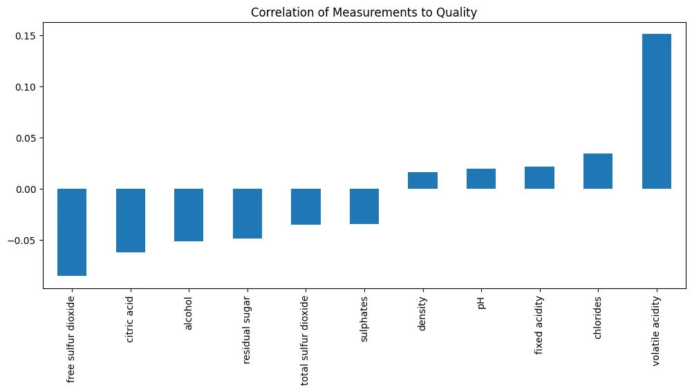
Regression Model

# separate target + remove string values
X_wine = wine_df.drop(['quality_enc', 'quality', 'type'], axis=1)
y_wine = wine_df['quality']

print(X_wine.shape, y_wine.shape)

# train-test split
X_wine_train, X_wine_test, y_wine_train, y_wine_test = train_test_split(
    X_wine,
    y_wine,
    test_size=0.1,
    random_state=42
)

# normalization
scaler = StandardScaler()
X_wine_train_scaled = scaler.fit_transform(X_wine_train)
X_wine_test_scaled = scaler.transform(X_wine_test)

# create the SVC model using class_weight to balance out the
# dataset that heavily leaning towards non-frauds
svc_wine_base = svm.SVC(
    kernel='rbf',
    class_weight='balanced'
)

# grid search
param_grid = \{
    'C': [0.5, 1, 1.5, 2, 2.5],
    'gamma' : ['scale', 'auto']
\}

wine_grid = GridSearchCV(svc_wine_base, param_grid)
wine_grid.fit(X_wine_train_scaled, y_wine_train)
print('Best Params: ', wine_grid.best_params_)
# Best Params:  \{'C': 2.5, 'gamma': 'auto'\}

y_wine_pred = wine_grid.predict(X_wine_test_scaled)

print(
    'Accuracy Score: ',
    accuracy_score(y_wine_test, y_wine_pred, normalize=True).round(4)*100, '%'
)
# Accuracy Score:  84.77 %

report_wine = classification_report(
    y_wine_test, y_wine_pred
)
print(report_wine)

	precision	recall	f1-score	support
Fraud	0.16	0.68	0.26	25
Legit	0.99	0.85	0.92	625
accuracy			0.85	650
macro avg	0.57	0.77	0.59	650
weighted avg	0.95	0.85	0.89	650

conf_mtx_wine = confusion_matrix(y_wine_test, y_wine_pred)
conf_mtx_wine

# array([[ 17,   8],
#        [ 91, 534]])

conf_mtx_wine_plot = ConfusionMatrixDisplay(
    confusion_matrix=conf_mtx_wine
)

conf_mtx_wine_plot.plot(cmap='plasma')

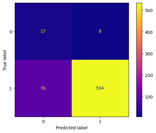
# expand grid search
param_grid = \{
    'C': [1000, 1050, 1100, 1050, 1200],
    'gamma' : ['scale', 'auto']
\}

wine_grid = GridSearchCV(svc_wine_base, param_grid)
wine_grid.fit(X_wine_train_scaled, y_wine_train)
print('Best Params: ', wine_grid.best_params_)
# Best Params:  \{'C': 1100, 'gamma': 'scale'\}

y_wine_pred = wine_grid.predict(X_wine_test_scaled)
print('Accuracy Score: ',accuracy_score(y_wine_test, y_wine_pred, normalize=True).round(4)*100, '%')
# Accuracy Score:  94.31 %
report_wine = classification_report(y_wine_test, y_wine_pred)
print(report_wine)
conf_mtx_wine = confusion_matrix(y_wine_test, y_wine_pred)

conf_mtx_wine_plot = ConfusionMatrixDisplay(
    confusion_matrix=conf_mtx_wine
)

conf_mtx_wine_plot.plot(cmap='plasma')

	precision	recall	f1-score	support
Fraud	0.29	0.32	0.30	25
Legit	0.97	0.97	0.97	625
accuracy			0.85	650
macro avg	0.63	0.64	0.64	650
weighted avg	0.95	0.94	0.94	650

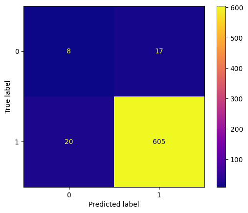
Supervised Learning - Boosting Methods

# dataset - label mushrooms as poisonous or eatable
!wget https://github.com/semnan-university-ai/Mushroom/raw/main/Mushroom.csv -P datasets

Dataset Exploration

shroom_df = pd.read_csv('datasets/mushrooms.csv')
shroom_df.head(5).transpose()

Mushroom Data Set

1. cap-shape: bell = b, conical = c, convex = x, flat = f, knobbed = k, sunken = s
2. cap-surface: fibrous = f, grooves = g, scaly = y, smooth = s
3. cap-color: brown = n, buff = b, cinnamon = c, gray = g, green = r, pink = p, purple = u, red = e, white = w, yellow = y
4. bruises?: bruises = t, no = f
5. odor: almond = a, anise = l, creosote = c, fishy = y, foul = f, musty = m, none = n, pungent = p, spicy = s
6. gill-attachment: attached = a, descending = d, free = f, notched = n
7. gill-spacing: close = c, crowded = w, distant = d
8. gill-size: broad = b, narrow = n
9. gill-color: black = k, brown = n, buff = b, chocolate = h, gray = g, green = r, orange = o, pink = p, purple = u, red = e, white = w, yellow = y
10. stalk-shape: enlarging = e, tapering = t
11. stalk-root: bulbous = b, club = c, cup = u, equal = e, rhizomorphs = z, rooted = r, missing = ?
12. stalk-surface-above-ring: fibrous = f, scaly = y, silky = k, smooth = s
13. stalk-surface-below-ring: fibrous = f, scaly = y, silky = k, smooth = s
14. stalk-color-above-ring: brown = n, buff = b, cinnamon = c, gray = g, orange = o, pink = p, red = e, white = w, yellow = y
15. stalk-color-below-ring: brown = n, buff = b, cinnamon = c, gray = g, orange = o, pink = p, red = e, white = w, yellow = y
16. veil-type: partial = p, universal = u
17. veil-color: brown = n, orange = o, white = w, yellow = y
18. ring-number: none = n, one = o, two = t
19. ring-type: cobwebby = c, evanescent = e, flaring = f, large = l, none = n, pendant = p, sheathing = s, zone = z
20. spore-print-color: black = k, brown = n, buff = b, chocolate = h, green = r, orange = o, purple = u, white = w, yellow = y
21. population: abundant = a, clustered = c, numerous = n, scattered = s, several = v, solitary = `y
22. habitat: grasses = g, leaves = l, meadows = m, paths = p, urban = u, waste = w, woods = d

	0	1	2	3	4
class	p	e	e	p	e
cap-shape	x	x	b	x	x
cap-surface	s	s	s	y	s
cap-color	n	y	w	w	g
bruises	t	t	t	t	f
odor	p	a	l	p	n
gill-attachment	f	f	f	f	f
gill-spacing	c	c	c	c	w
gill-size	n	b	b	n	b
gill-color	k	k	n	n	k
stalk-shape	e	e	e	e	t
stalk-root	e	c	c	e	e
stalk-surface-above-ring	s	s	s	s	s
stalk-surface-below-ring	s	s	s	s	s
stalk-color-above-ring	w	w	w	w	w
stalk-color-below-ring	w	w	w	w	w
veil-type	p	p	p	p	p
veil-color	w	w	w	w	w
ring-number	o	o	o	o	o
ring-type	p	p	p	p	e
spore-print-color	k	n	n	k	n
population	s	n	n	s	a
habitat	u	g	m	u	g

shroom_df.isnull().sum()

class	0
cap-shape	0
cap-surface	0
cap-color	0
bruises	0
odor	0
gill-attachment	0
gill-spacing	0
gill-size	0
gill-color	0
stalk-shape	0
stalk-root	0
stalk-surface-above-ring	0
stalk-surface-below-ring	0
stalk-color-above-ring	0
stalk-color-below-ring	0
veil-type	0
veil-color	0
ring-number	0
ring-type	0
spore-print-color	0
population	0
habitat	0
dtype: int64

feature_df = shroom_df.describe().transpose().reset_index(
    names=['feature']
).sort_values(
    'unique', ascending=False
)

	feature	count	unique	top	freq
9	gill-color	8124	12	b	1728
3	cap-color	8124	10	n	2284
20	spore-print-color	8124	9	w	2388
5	odor	8124	9	n	3528
15	stalk-color-below-ring	8124	9	w	4384
14	stalk-color-above-ring	8124	9	w	4464
22	habitat	8124	7	d	3148
1	cap-shape	8124	6	x	3656
21	population	8124	6	v	4040
19	ring-type	8124	5	p	3968
11	stalk-root	8124	5	b	3776
12	stalk-surface-above-ring	8124	4	s	5176
13	stalk-surface-below-ring	8124	4	s	4936
17	veil-color	8124	4	w	7924
2	cap-surface	8124	4	y	3244
18	ring-number	8124	3	o	7488
10	stalk-shape	8124	2	t	4608
8	gill-size	8124	2	b	5612
7	gill-spacing	8124	2	c	6812
6	gill-attachment	8124	2	f	7914
4	bruises	8124	2	f	4748
0	class	8124	2	e	4208
16	veil-type	8124	1	p	8124

plt.figure(figsize=(12,8))
plt.title('Mushroom Features :: Number of unique Features')
sns.barplot(data=feature_df, y='feature', x='unique', orient='h', palette='summer_r')

plt.figure(figsize=(10,4))
plt.title('Mushroom Count :: Editable vs Poisonous')
sns.countplot(data=shroom_df, x='class', palette='seismic_r')

Adaptive Boosting

# remove lable class
X_shroom = shroom_df.drop('class', axis=1)
# make all values numeric
X_shroom = pd.get_dummies(X_shroom, drop_first=True)

y_shroom = shroom_df['class']

# train/test split
X_shroom_train, X_shroom_test, y_shroom_train, y_shroom_test = train_test_split(
    X_shroom,
    y_shroom,
    test_size=0.15,
    random_state=42
)

Feature Exploration

# don't try fit a perfect model but only return
# the most important feature for classification
abc_shroom = AdaBoostClassifier(estimator=None, n_estimators=1)
abc_shroom.fit(X_shroom_train,y_shroom_train)

shroom_preds = abc_shroom.predict(X_shroom_test)

print('Accuracy Score: ',accuracy_score(y_shroom_test, shroom_preds, normalize=True).round(4)*100, '%')
# Accuracy Score:  88.35 %

report_shroom = classification_report(y_shroom_test, shroom_preds)
print(report_shroom)

	precision	recall	f1-score	support
e	0.97	0.80	0.88	637
p	0.82	0.97	0.89	582
accuracy			0.88	1219
macro avg	0.89	0.89	0.88	1219
weighted avg	0.90	0.88	0.88	1219

conf_mtx_shroom = confusion_matrix(y_shroom_test, shroom_preds)

conf_mtx_shroom_plot = ConfusionMatrixDisplay(
    confusion_matrix=conf_mtx_shroom
)

conf_mtx_shroom_plot.plot(cmap='winter_r')

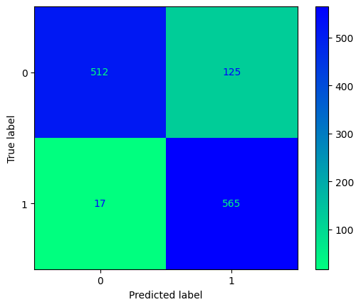
# the model was fit on a single feature and still resulted in a pretty good performance.
# Let's find out what feature was chosen for the classification.

shroom_index = ['importance']
shroom_data_columns = pd.Series(X_shroom.columns)
shroom_importance_array = abc_shroom.feature_importances_
shroom_importance_df = pd.DataFrame(shroom_importance_array, shroom_data_columns, shroom_index)
shroom_importance_df.value_counts()

importance	count
0.0	94
1.0	1
dtype: int64

# plot a slice of the dataframe to find the feature
shroom_importance_df_sorted = shroom_importance_df.sort_values(
    by='importance',
    ascending=True
)

shroom_importance_df_sorted[-5:].plot(
    kind='barh',
    title='Feature Importance for Mushroom Classification',
    figsize=(8,4)
)

The most important feature (as determined by the model) is the odor - in this case a odor of none is the best indicator to classify a poisonous mushroom:

odor: almond = a, anise = l, creosote = c, fishy = y, foul = f, musty = m, none = n, pungent = p, spicy = s

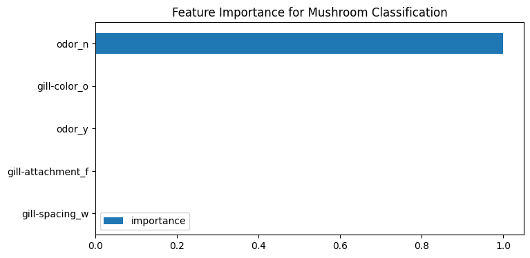
# the mojority of poisonous mushrooms do have an odor
# naking the lack of it a good indicator for an eatable variety
plt.figure(figsize=(12,4))
plt.title('Mushroom Odor vs Class')
sns.countplot(data=shroom_df, x='odor', hue='class', palette='summer')

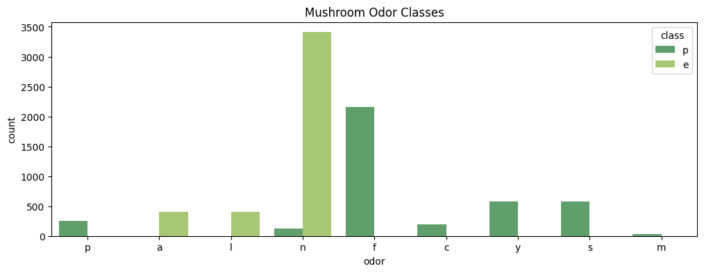
Optimizing Hyperparameters

# find out how many of the 95 features you have
# to add to your model to get a better fit

error_rates = []

for estimators in range(1,96):
    model = AdaBoostClassifier(n_estimators=estimators)
    model.fit(X_shroom_train,y_shroom_train)
    preds = model.predict(X_shroom_test)
    
    err = 1 - accuracy_score(y_shroom_test, preds)
    error_rates.append(err)

x_range=range(1,96)
plt.figure(figsize=(10,4))
plt.title('Adaboost Error Rate vs n_estimators')
plt.xlabel('n_estimators')
plt.ylabel('Error Rate')
plt.xticks(np.arange(min(x_range), max(x_range)+1, 3.0))
plt.plot(x_range, error_rates)

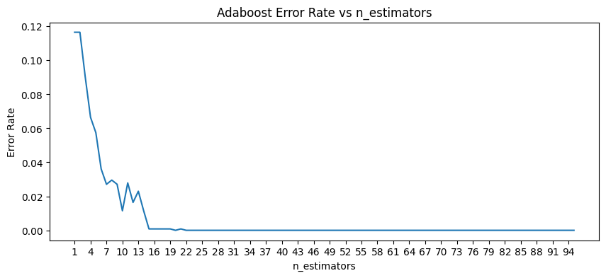
# already after 16 estimators there is no
# visible improvment for the error rate
abc_shroom2 = AdaBoostClassifier(estimator=None, n_estimators=16)
abc_shroom2.fit(X_shroom_train,y_shroom_train)

shroom_preds2 = abc_shroom2.predict(X_shroom_test)

print('Accuracy Score: ',accuracy_score(y_shroom_test, shroom_preds2, normalize=True).round(4)*100, '%')
# Accuracy Score:  99.92 %

report_shroom2 = classification_report(y_shroom_test, shroom_preds2)
print(report_shroom2)

	precision	recall	f1-score	support
e	1.00	1.00	1.00	637
p	1.00	1.00	1.00	582
accuracy			1.00	1219
macro avg	1.00	1.00	1.00	1219
weighted avg	1.00	1.00	1.00	1219

conf_mtx_shroom2 = confusion_matrix(y_shroom_test, shroom_preds2)

conf_mtx_shroom_plot2 = ConfusionMatrixDisplay(
    confusion_matrix=conf_mtx_shroom2
)

conf_mtx_shroom_plot2.plot(cmap='winter_r')

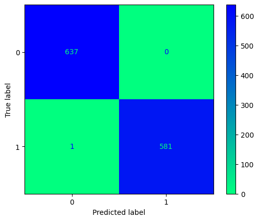
shroom_index = ['importance']
shroom_data_columns = pd.Series(X_shroom.columns)
shroom_importance_array = abc_shroom2.feature_importances_
shroom_importance_df = pd.DataFrame(shroom_importance_array, shroom_data_columns, shroom_index)
shroom_importance_df.value_counts()

# there are 12 features now that are deemed important

importance	count
0.0000	83
0.0625	9
0.1250	2
0.1875	1
dtype: int64

shroom_importance_df_sorted = shroom_importance_df.sort_values(
    by='importance',
    ascending=True
).tail(13)

	importance
gill-size_n	0.1875
population_v	0.1250
odor_n	0.1250
odor_c	0.0625
stalk-shape_t	0.0625
spore-print-color_w	0.0625
population_c	0.0625
ring-type_p	0.0625
spore-print-color_r	0.0625
stalk-surface-above-ring_k	0.0625
gill-spacing_w	0.0625
odor_f	0.0625
stalk-color-below-ring_w	0.0000

plt.figure(figsize=(10,6))
plt.title('Features important to classify poisonous Mushrooms')

sns.barplot(
    data=shroom_importance_df_sorted.tail(13),
    y=shroom_importance_df_sorted.tail(13).index,
    x='importance',
    orient='h',
    palette='summer'
)

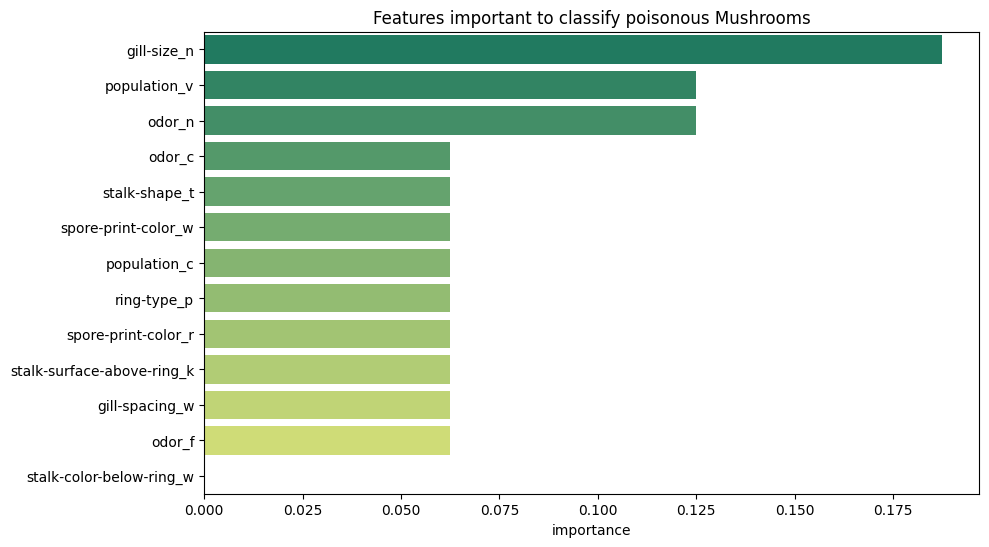
Gradient Boosting

Gridsearch for best Hyperparameter

gb_shroom = GradientBoostingClassifier()

param_grid = \{
    'n_estimators': [50, 100, 150],
    'learning_rate': [0.05,0.1,0.2],
    'max_depth': [2,3,4,5]
\}

shroom_grid = GridSearchCV(gb_shroom, param_grid)
shroom_grid.fit(X_shroom_train, y_shroom_train)
shroom_grid.best_params_
# \{'learning_rate': 0.05, 'max_depth': 4, 'n_estimators': 150\}

shroom_grid_preds = shroom_grid.predict(X_shroom_test)

print('Accuracy Score: ',accuracy_score(y_shroom_test, shroom_grid_preds, normalize=True).round(4)*100, '%')
# Accuracy Score:  100.0 %

report_shroom_grid_preds = classification_report(y_shroom_test, shroom_grid_preds)
print(report_shroom_grid_preds)

	precision	recall	f1-score	support
e	1.00	1.00	1.00	637
p	1.00	1.00	1.00	582
accuracy			1.00	1219
macro avg	1.00	1.00	1.00	1219
weighted avg	1.00	1.00	1.00	1219

conf_mtx_shroom_grid = confusion_matrix(y_shroom_test, shroom_grid_preds)

conf_mtx_shroom_grid_plot = ConfusionMatrixDisplay(
    confusion_matrix=conf_mtx_shroom_grid
)

conf_mtx_shroom_grid_plot.plot(cmap='winter_r')

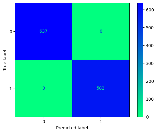
Feature Importance

shroom_feature_importance = shroom_grid.best_estimator_.feature_importances_
feature_importance_df = pd.DataFrame(
    index = X_shroom.columns,
    data = shroom_feature_importance,
    columns = ['importance']
)

# kick all features that have zero importance and sort by importance
feature_importance_df = feature_importance_df[
    feature_importance_df['importance'] > 3e-03
].sort_values(
    by='importance',
    ascending=False
)

plt.figure(figsize=(10,6))
plt.title('Features important to classify poisonous Mushrooms')

sns.barplot(
    data=feature_importance_df,
    y=feature_importance_df.index,
    x='importance',
    orient='h',
    palette='summer'
)

Supervised Learning - Naive Bayes NLP

Feature Extraction

text = [
    'This is a dataset for binary sentiment classification',
    'containing substantially more data than previous benchmark datasets',
    'We provide a set of 25,000 highly polar movie reviews for training',
    'And 25,000 for testing',
    'There is additional unlabeled data for use as well',
    'Raw text and already processed bag of words formats are provided'
]

CountVectorizer & TfidfTransformer

cv = CountVectorizer(stop_words='english')
cv_sparse_matrix = cv.fit_transform(text)
# <6x30 sparse matrix of type '<class 'numpy.int64'>'
# 	with 33 stored elements in Compressed Sparse Row format>

print(cv_sparse_matrix.todense())
# [[0 0 0 0 0 1 1 0 0 1 0 0 0 0 0 0 0 0 0 0 0 1 0 0 0 0 0 0 0 0]
#  [0 0 0 0 1 0 0 1 1 0 1 0 0 0 0 1 0 0 0 0 0 0 0 1 0 0 0 0 0 0]
#  [1 1 0 0 0 0 0 0 0 0 0 0 1 1 1 0 0 1 0 0 1 0 1 0 0 0 1 0 0 0]
#  [1 1 0 0 0 0 0 0 0 0 0 0 0 0 0 0 0 0 0 0 0 0 0 0 1 0 0 0 0 0]
#  [0 0 1 0 0 0 0 0 1 0 0 0 0 0 0 0 0 0 0 0 0 0 0 0 0 0 0 1 1 0]
#  [0 0 0 1 0 0 0 0 0 0 0 1 0 0 0 0 1 0 1 1 0 0 0 0 0 1 0 0 0 1]]

print(cv.vocabulary_)
# \{'dataset': 9, 'binary': 5, 'sentiment': 21, 'classification': 6, 'containing': 7, 'substantially': 23, 'data': 8, 'previous': 15, 'benchmark': 4, 'datasets': 10, 'provide': 17, 'set': 22, '25': 1, '000': 0, 'highly': 12, 'polar': 14, 'movie': 13, 'reviews': 20, 'training': 26, 'testing': 24, 'additional': 2, 'unlabeled': 27, 'use': 28, 'raw': 19, 'text': 25, 'processed': 16, 'bag': 3, 'words': 29, 'formats': 11, 'provided': 18\}

tfidf_trans = TfidfTransformer()
tfidf_trans_results = tfidf_trans.fit_transform(cv_sparse_matrix)

print(tfidf_trans_results.todense())
# [[0.         0.         0.         0.         0.         0.5
#   0.5        0.         0.         0.5        0.         0.
#   0.         0.         0.         0.         0.         0.
#   0.         0.         0.         0.5        0.         0.
#   0.         0.         0.         0.         0.         0.        ]
#  [0.         0.         0.         0.         0.4198708  0.
#   0.         0.4198708  0.34430007 0.         0.4198708  0.
#   0.         0.         0.         0.4198708  0.         0.
#   0.         0.         0.         0.         0.         0.4198708
#   0.         0.         0.         0.         0.         0.        ]
#  [0.28386526 0.28386526 0.         0.         0.         0.
#   0.         0.         0.         0.         0.         0.
#   0.3461711  0.3461711  0.3461711  0.         0.         0.3461711
#   0.         0.         0.3461711  0.         0.3461711  0.
#   0.         0.         0.3461711  0.         0.         0.        ]
#  [0.5355058  0.5355058  0.         0.         0.         0.
#   0.         0.         0.         0.         0.         0.
#   0.         0.         0.         0.         0.         0.
#   0.         0.         0.         0.         0.         0.
#   0.65304446 0.         0.         0.         0.         0.        ]
#  [0.         0.         0.52182349 0.         0.         0.
#   0.         0.         0.42790272 0.         0.         0.
#   0.         0.         0.         0.         0.         0.
#   0.         0.         0.         0.         0.         0.
#   0.         0.         0.         0.52182349 0.52182349 0.        ]
#  [0.         0.         0.         0.37796447 0.         0.
#   0.         0.         0.         0.         0.         0.37796447
#   0.         0.         0.         0.         0.37796447 0.
#   0.37796447 0.37796447 0.         0.         0.         0.
#   0.         0.37796447 0.         0.         0.         0.37796447]]

TfidfVectorizer

tfidf_vec = TfidfVectorizer(
    lowercase=True,
    analyzer='word',
    stop_words='english'
)

tfidf_vec_results = tfidf_vec.fit_transform(text)
# <6x30 sparse matrix of type '<class 'numpy.float64'>'
# 	with 33 stored elements in Compressed Sparse Row format>

print(tfidf_trans_results == tfidf_vec_results)
# True

Dataset Exploration

!wget https://raw.githubusercontent.com/kunal-lalwani/Twitter-US-Airlines-Sentiment-Analysis/master/Tweets.csv -P datasets

tweet_df = pd.read_csv('datasets/Tweets.csv')
tweet_df.head(3).transpose()

	0	1	2
tweet_id	570306133677760513	570301130888122368	570301083672813571
airline_sentiment	neutral	positive	neutral
airline_sentiment_confidence	1.0	0.3486	0.6837
negativereason	NaN	NaN	NaN
negativereason_confidence	NaN	0.0	NaN
airline	Virgin America	Virgin America	Virgin America
airline_sentiment_gold	NaN	NaN	NaN
name	cairdin	jnardino	yvonnalynn
negativereason_gold	NaN	NaN	NaN
retweet_count	0	0	0
text	@VirginAmerica What @dhepburn said.	@VirginAmerica plus you've added commercials t...	@VirginAmerica I didn't today... Must mean I n...
tweet_coord	NaN	NaN	NaN
tweet_created	2015-02-24 11:35:52 -0800	2015-02-24 11:15:59 -0800	2015-02-24 11:15:48 -0800
tweet_location	NaN	NaN	Lets Play
user_timezone	Eastern Time (US & Canada)	Pacific Time (US & Canada)	Central Time (US & Canada)

plt.figure(figsize=(12,5))
plt.title('Tweet Sentiment Classification by Airline')
sns.countplot(
    data=tweet_df,
    x='airline',
    hue='airline_sentiment',
    palette='cool'
)

plt.savefig('assets/Scikit_Learn_56.webp', bbox_inches='tight')

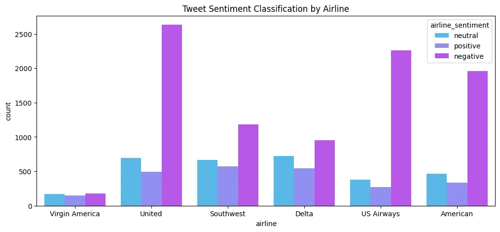
plt.figure(figsize=(12,6))
plt.title('Tweet Sentiment Classification with negative Reason')
sns.countplot(
    data=tweet_df,
    x='airline',
    hue='negativereason',
    palette='cool'
)

plt.savefig('assets/Scikit_Learn_57.webp', bbox_inches='tight')

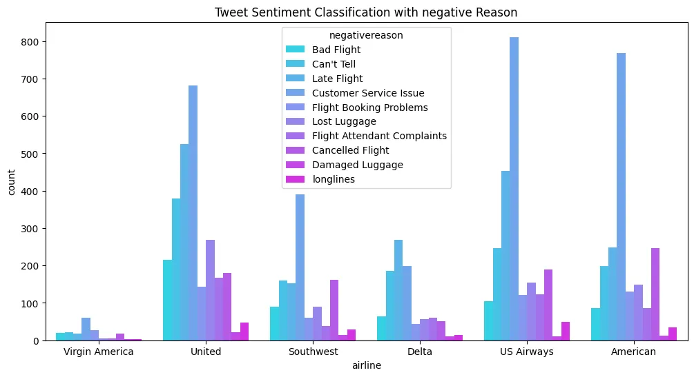
Data Preprocessing

tweet_data = tweet_df[['airline_sentiment', 'text']]

X_tweet = tweet_data['text']
y_tweet = tweet_data['airline_sentiment']

# train/ test split
X_tweet_train, X_tweet_test, y_tweet_train, y_tweet_test = train_test_split(
    X_tweet,
    y_tweet,
    test_size=0.2,
    random_state=42
)

TFIDF Vectorizer

tfidf_tweet_vec = TfidfVectorizer(
    lowercase=True,
    analyzer='word',
    stop_words='english'
)

X_tweet_tfidf_train = tfidf_tweet_vec.fit_transform(X_tweet_train)
# <11712x12987 sparse matrix of type '<class 'numpy.float64'>'
# 	with 106745 stored elements in Compressed Sparse Row format>
X_tweet_tfidf_test = tfidf_tweet_vec.transform(X_tweet_test)

Model Comparison

# report helper function
def report(model):
    preds = model.predict(X_tweet_tfidf_test)
    
    print(classification_report(y_tweet_test, preds))
    
    conf_mtx = confusion_matrix(y_tweet_test, preds)
    conf_mtx_plot = ConfusionMatrixDisplay(
        confusion_matrix=conf_mtx
    )
    conf_mtx_plot.plot(cmap='plasma')

logreg_tweet = LogisticRegression(max_iter=1000)
logreg_tweet.fit(X_tweet_tfidf_train, y_tweet_train)

report(logreg_tweet)

	precision	recall	f1-score	support
negative	0.82	0.93	0.88	1889
neutral	0.66	0.48	0.56	580
positive	0.79	0.63	0.70	459
accuracy			0.80	2928
macro avg	0.76	0.68	0.71	2928
weighted avg	0.79	0.80	0.78	2928

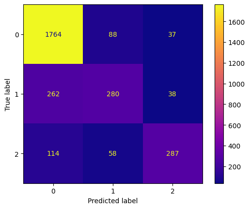
rbf_svc_tweet = svm.SVC()
rbf_svc_tweet.fit(X_tweet_tfidf_train, y_tweet_train)

report(rbf_svc_tweet)

	precision	recall	f1-score	support
negative	0.81	0.95	0.87	1889
neutral	0.68	0.42	0.52	580
positive	0.80	0.61	0.69	459
accuracy			0.79	2928
macro avg	0.76	0.66	0.69	2928
weighted avg	0.78	0.79	0.77	2928

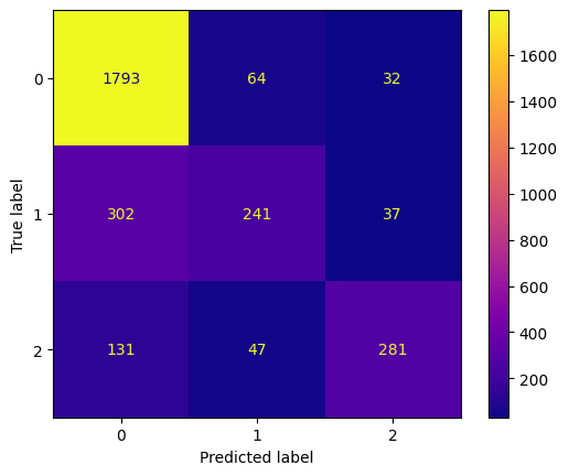
linear_svc_tweet = svm.LinearSVC()
linear_svc_tweet.fit(X_tweet_tfidf_train, y_tweet_train)

report(linear_svc_tweet)

	precision	recall	f1-score	support
negative	0.85	0.91	0.88	1889
neutral	0.64	0.54	0.58	580
positive	0.76	0.67	0.71	459
accuracy			0.80	2928
macro avg	0.75	0.71	0.72	2928
weighted avg	0.79	0.80	0.79	2928

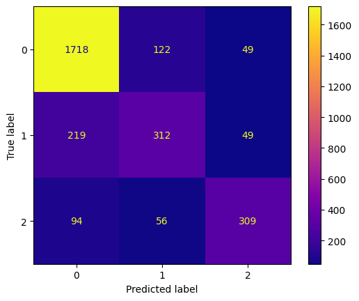
nb_tweets = MultinomialNB()
nb_tweets.fit(X_tweet_tfidf_train, y_tweet_train)

report(nb_tweets)
# The Naive Bayes classifies almost all tweets as negative
# which means it does well with searching neg tweets
# but ends up classifying a lot neutral and pos tweets as neg

	precision	recall	f1-score	support
negative	0.69	0.99	0.81	1889
neutral	0.75	0.15	0.25	580
positive	0.94	0.18	0.31	459
accuracy			0.70	2928
macro avg	0.79	0.44	0.46	2928
weighted avg	0.74	0.70	0.62	2928

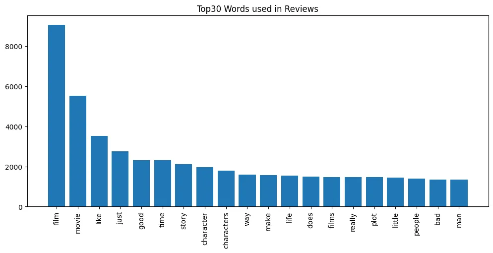
Model Deployment

# building a pipeline to ingest new tweets with the best performing model
pipe = Pipeline(
    [
        ('tfidf', TfidfVectorizer()),
        ('svc', svm.SVC())
    ]
)

# before deployment retrain on entire dataset
pipe.fit(X_tweet, y_tweet)

# test prediction
print(pipe.predict([
    'good flight',
    'terrible service',
    'too late',
    'ok flight',
    'Thank you'
]))
# ['positive' 'negative' 'negative' 'neutral' 'positive']

Text Classification

IMDB Dataset of 50K Movie Reviews https://ai.stanford.edu/~amaas/data/sentiment/

Data Exploration

imdb_df = pd.read_csv('datasets/moviereviews.csv')
imdb_df.head()

	label	review
0	neg	how do films like mouse hunt get into theatres...
1	neg	some talented actresses are blessed with a dem...
2	pos	this has been an extraordinary year for austra...
3	pos	according to hollywood movies made in last few...
4	neg	my first press screening of 1998 and already i...

imdb_df.info()

# <class 'pandas.core.frame.DataFrame'>
# RangeIndex: 2000 entries, 0 to 1999
# Data columns (total 2 columns):
#  #   Column  Non-Null Count  Dtype 
# ---  ------  --------------  ----- 
#  0   label   2000 non-null   object
#  1   review  1965 non-null   object
# dtypes: object(2)
# memory usage: 31.4+ KB

# find missing
imdb_df.isnull().sum()
# label      0
# review    35
# dtype: int64

# drop missing
imdb_df = imdb_df.dropna(axis=0)
imdb_df.isnull().sum()
# label     0
# review    0
# dtype: int64

# make sure there a no empty string reviews
# (imdb_df['review'] == '  ').sum()
imdb_df['review'].str.isspace().sum()
# 27

# remove empty string reviews
imdb_df = imdb_df[~imdb_df['review'].str.isspace()]
imdb_df = imdb_df[imdb_df['review'] != '']

imdb_df['review'].str.isspace().sum()
# 0

# is the dataset balanced
imdb_df['label'].value_counts()
# neg    969
# pos    969
# Name: label, dtype: int64

Top 30 Features by Label

# find top 20 words in negative reviews
imdb_neg_df = imdb_df[imdb_df['label'] == 'neg']

count_vectorizer = CountVectorizer(analyzer='word', stop_words='english')
bag_of_words = count_vectorizer.fit_transform(imdb_neg_df['review'])
sum_words = bag_of_words.sum(axis=0)

words_freq = [
    (word, sum_words[0, idx]) for word, idx in count_vectorizer.vocabulary_.items()
]

words_freq =sorted(words_freq, key = lambda x: x[1], reverse=True)

x, y = zip(*words_freq[:30])

plt.figure(figsize=(12,5))
plt.bar(x,y)
plt.xticks(rotation=90)
plt.title('Top30 Words used in Negative Reviews')

plt.savefig('assets/Scikit_Learn_62.webp', bbox_inches='tight')

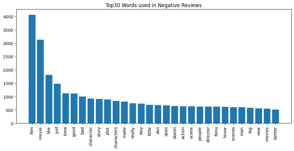
# find top 20 words in positive reviews
imdb_pos_df = imdb_df[imdb_df['label'] != 'neg']

count_vectorizer = CountVectorizer(analyzer='word', stop_words='english')
bag_of_words = count_vectorizer.fit_transform(imdb_pos_df['review'])
sum_words = bag_of_words.sum(axis=0)

words_freq = [
    (word, sum_words[0, idx]) for word, idx in count_vectorizer.vocabulary_.items()
]

words_freq =sorted(words_freq, key = lambda x: x[1], reverse=True)

x, y = zip(*words_freq[:30])

plt.figure(figsize=(12,5))
plt.bar(x,y)
plt.xticks(rotation=90)
plt.title('Top30 Words used in Positive Reviews')

plt.savefig('assets/Scikit_Learn_63.webp', bbox_inches='tight')

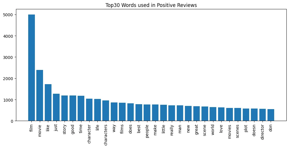
Data Preprocessing

X_rev = imdb_df['review']
y_rev = imdb_df['label']

# train/ test split
X_rev_train, X_rev_test, y_rev_train, y_rev_test = train_test_split(
    X_rev,
    y_rev,
    test_size=0.2,
    random_state=42
)

tfidf_rev_vec = TfidfVectorizer(
    lowercase=True,
    analyzer='word',
    stop_words='english'
)

X_rev_tfidf_train = tfidf_rev_vec.fit_transform(X_rev_train)
X_rev_tfidf_test = tfidf_rev_vec.transform(X_rev_test)

Model Training

nb_rev = MultinomialNB()
nb_rev.fit(X_rev_tfidf_train, y_rev_train)

preds = nb_rev.predict(X_rev_tfidf_test)
print(classification_report(y_rev_test, preds))

	precision	recall	f1-score	support
neg	0.79	0.88	0.83	188
pos	0.87	0.78	0.82	200
accuracy			0.82	388
macro avg	0.83	0.83	0.82	388
weighted avg	0.83	0.82	0.82	388

conf_mtx = confusion_matrix(y_rev_test, preds)
conf_mtx_plot = ConfusionMatrixDisplay(
     confusion_matrix=conf_mtx
)
conf_mtx_plot.plot(cmap='plasma')

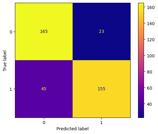
Unsupervised Learning - KMeans Clustering

Dataset Exploration

!wget https://github.com/selva86/datasets/raw/master/bank-full.csv -P datasets

bank_df = pd.read_csv('datasets/bank-full.csv', sep=';')
bank_df.head(5).transpose()

	0	1	2	3	4
age	56	57	37	40	56
job	housemaid	services	services	admin.	services
marital	married	married	married	married	married
education	basic.4y	high.school	high.school	basic.6y	high.school
default	no	unknown	no	no	no
housing	no	no	yes	no	no
loan	no	no	no	no	yes
contact	telephone	telephone	telephone	telephone	telephone
month	may	may	may	may	may
day_of_week	mon	mon	mon	mon	mon
duration	261	149	226	151	307
campaign	1	1	1	1	1
pdays	999	999	999	999	999
previous	0	0	0	0	0
poutcome	nonexistent	nonexistent	nonexistent	nonexistent	nonexistent
emp.var.rate	1.1	1.1	1.1	1.1	1.1
cons.price.idx	93.994	93.994	93.994	93.994	93.994
cons.conf.idx	-36.4	-36.4	-36.4	-36.4	-36.4
euribor3m	4.857	4.857	4.857	4.857	4.857
nr.employed	5191.0	5191.0	5191.0	5191.0	5191.0
y	no	no	no	no	no

bank_df.describe()

	age	duration	campaign	pdays	previous	emp.var.rate	cons.price.idx	cons.conf.idx	euribor3m	nr.employed
count	41188.00000	41188.000000	41188.000000	41188.000000	41188.000000	41188.000000	41188.000000	41188.000000	41188.000000	41188.000000
mean	40.02406	258.285010	2.567593	962.475454	0.172963	0.081886	93.575664	-40.502600	3.621291	5167.035911
std	10.42125	259.279249	2.770014	186.910907	0.494901	1.570960	0.578840	4.628198	1.734447	72.251528
min	17.00000	0.000000	1.000000	0.000000	0.000000	-3.400000	92.201000	-50.800000	0.634000	4963.600000
25%	32.00000	102.000000	1.000000	999.000000	0.000000	-1.800000	93.075000	-42.700000	1.344000	5099.100000
50%	38.00000	180.000000	2.000000	999.000000	0.000000	1.100000	93.749000	-41.800000	4.857000	5191.000000
75%	47.00000	319.000000	3.000000	999.000000	0.000000	1.400000	93.994000	-36.400000	4.961000	5228.100000
max	98.00000	4918.000000	56.000000	999.000000	7.000000	1.400000	94.767000	-26.900000	5.045000	5228.100000

plt.figure(figsize=(12, 5))
plt.title('Age Distribution by Marital Status')

sns.histplot(
    data=bank_df,
    x='age',
    bins=50,
    hue='marital',
    palette='winter',
    kde=True
)

plt.savefig('assets/Scikit_Learn_65.webp', bbox_inches='tight')

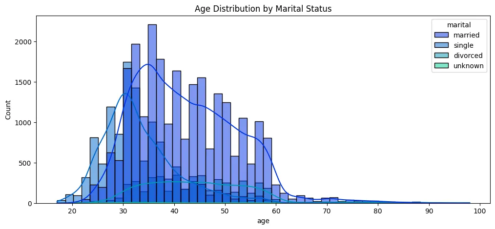
plt.figure(figsize=(12, 5))
plt.title('Age Distribution by Loan Status')

sns.histplot(
    data=bank_df,
    x='age',
    bins=50,
    hue='loan',
    palette='winter',
    kde=True
)

plt.savefig('assets/Scikit_Learn_66.webp', bbox_inches='tight')

# remove columns with `pday`s = 999 (placeholder for never)
plt.figure(figsize=(12, 5))
plt.title('Distribution of Days Since Last Contacted by Loan Status')

sns.histplot(
    data=bank_df[bank_df['pdays'] != 999],
    x='pdays',
    hue='loan',
    palette='winter',
    kde=True
)

plt.savefig('assets/Scikit_Learn_67.webp', bbox_inches='tight')

# Create call duration in minutes column
bank_df['duration_minutes'] = bank_df['duration'].apply(lambda x: x/60).round(1)

plt.figure(figsize=(12, 5))
plt.title('Distribution Contact Duration by Contact Type')
plt.xlim(0,20)
sns.histplot(
    data=bank_df,
    x='duration_minutes',
    hue='contact',
    palette='winter',
    kde=True
)

plt.savefig('assets/Scikit_Learn_68.webp', bbox_inches='tight')

plt.figure(figsize=(16, 5))
plt.title('Customer Jobs Countplot by Loan Defaults')
sns.countplot(
    data=bank_df,
    x='job',
    order=bank_df['job'].value_counts().index,
    palette='winter',
    hue='default'
)

plt.savefig('assets/Scikit_Learn_69.webp', bbox_inches='tight')

plt.figure(figsize=(16, 5))
plt.title('Customer Education Countplot by Loan Defaults')
sns.countplot(
    data=bank_df,
    x='education',
    order=bank_df['education'].value_counts().index,
    palette='winter',
    hue='default'
)

plt.savefig('assets/Scikit_Learn_70.webp', bbox_inches='tight')

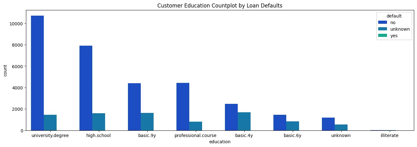
sns.pairplot(
    data=bank_df,
    hue='marital',
    palette='winter'
)

plt.savefig('assets/Scikit_Learn_71.webp', bbox_inches='tight')

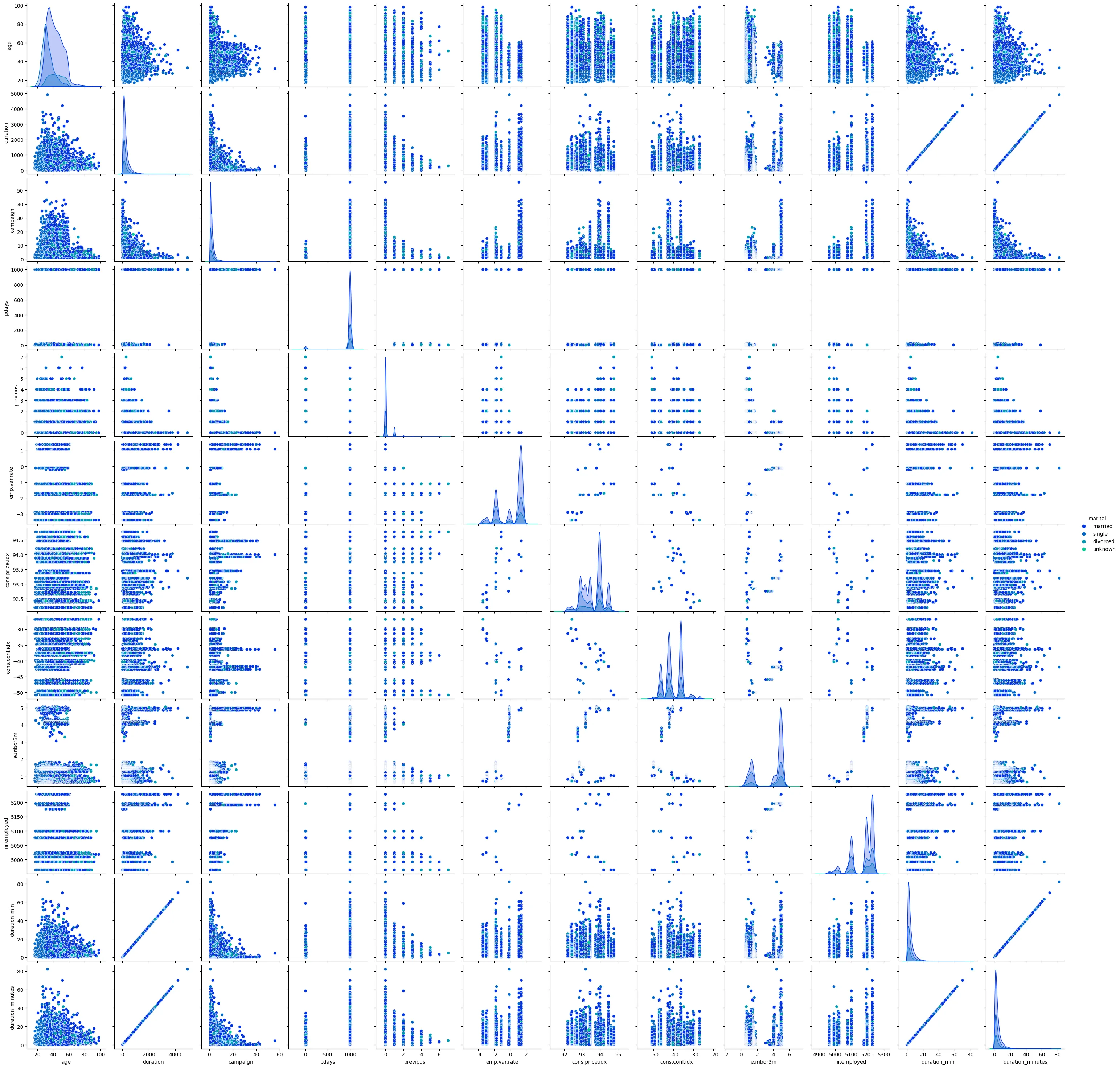
Dataset Preprocessing

# encode categorical features
X_bank = pd.get_dummies(bank_df)

# normalize data
bank_scaler = StandardScaler()

X_bank_scaled = bank_scaler.fit_transform(X_bank)

Model Training

bank_model = KMeans(
    n_clusters=2,
    n_init='auto',
    random_state=42
)
# fit to find cluster centers and predict what center every feature belongs to
bank_cluster_labels = bank_model.fit_predict(X_bank_scaled)

# add predicted label to source dataframe
X_bank['Cluster'] = bank_cluster_labels

X_bank['Cluster'].value_counts()
# 0    26871
# 1    14317
# Name: Cluster, dtype: int64

# How do the feature correlate with the predicted labels
label_corr = X_bank.corr()['Cluster']
print(label_corr.iloc[:-1].sort_values())

plt.figure(figsize=(10,14))
label_corr.iloc[:-1].sort_values().plot(kind='barh')
plt.title('Feature Importance')

plt.savefig('assets/Scikit_Learn_72.webp', bbox_inches='tight')

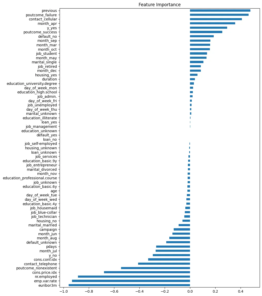
Choosing a K Value

# visualize the sum distance of your datapoints to the
# predicted cluster centers as a function of number of clusters
sum_squared_distance = []

for k in range(2,20):
    model = KMeans(n_clusters=k, n_init='auto')
    model.fit(X_bank_scaled)
    
    sum_squared_distance.append(model.inertia_)

plt.figure(figsize=(10,5))
plt.title('SSD as a Function of Number of Cluster')
plt.plot(range(2,20), sum_squared_distance, 'o--')

plt.savefig('assets/Scikit_Learn_73.webp', bbox_inches='tight')

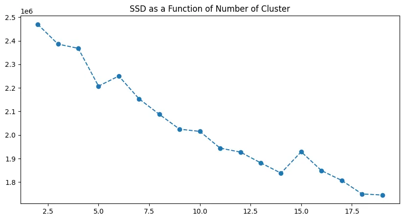
plt.figure(figsize=(10,5))
plt.title('Difference in SSD as a Function of Number of Clusters')
pd.Series(sum_squared_distance).diff().plot(kind='bar')

plt.savefig('assets/Scikit_Learn_74.webp', bbox_inches='tight')

There are two 'elbows' - one between k=5-6 (behold the 0-index in Pandas!) and the second one between k=14-15. Both of them are potential good values for the number of cluster k.

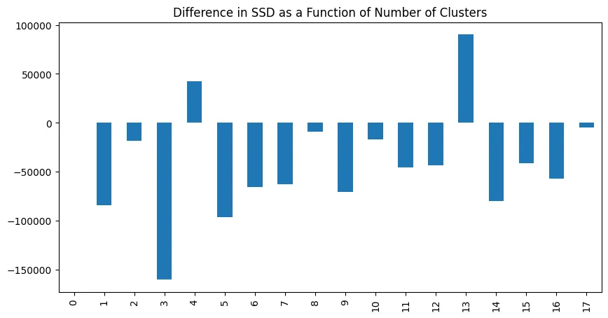
Re-fitting the Model

bank_model = KMeans(
    n_clusters=6,
    n_init='auto',
    random_state=42
)
# fit to find cluster centers and predict what center every feature belongs to
bank_cluster_labels = bank_model.fit_predict(X_bank_scaled)

# add predicted label to source dataframe
X_bank['Cluster'] = bank_cluster_labels
X_bank['Cluster'].value_counts()
# 5    10713
# 0    10663
# 1     8164
# 3     5566
# 4     3322
# 2     2760
# Name: Cluster, dtype: int64

Example 1 : Color Quantization

img_array = mpimg.imread('assets/gz.jpg')
img_array.shape
# (325, 640, 3)

plt.imshow(img_array)
plt.title('Original Image')
plt.savefig('assets/Scikit_Learn_75.webp', bbox_inches='tight')

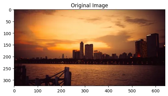
# flatten the image from 3 to 2 dimensions
(height, width, colour) = img_array.shape
img_array2d = img_array.reshape(height*width,colour)
img_array2d.shape
# (208000, 3)

# reduce colour space to 6 clusters
colour_model = KMeans(n_clusters=6, n_init='auto')
colour_labels = colour_model.fit_predict(img_array2d)

# get rgb value for each of the 6 cluster centers
rgb_colours = colour_model.cluster_centers_.round(0).astype(int)
rgb_colours
# array([[186, 111,  58],
#        [ 31,  11,  16],
#        [135,  72,  46],
#        [236, 157,  73],
#        [ 81,  40,  34],
#        [252, 199, 125]])

# assign these rgb values to each pixel within the cluster
# and reshape to original 3d array
quantized_image = np.reshape(rgb_colours[colour_labels],(height,width,colour))

plt.imshow(quantized_image)
plt.title('Quantized Image')
plt.savefig('assets/Scikit_Learn_76.webp', bbox_inches='tight')

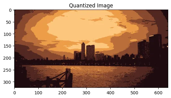
Example 2 : Country Clustering

Dataset Exploration

!wget https://github.com/priyansh21112002/CIA-Country-Description/raw/main/CIA_Country_Facts.csv -P datasets

country_df = pd.read_csv('datasets/CIA_Country_Facts.csv')
country_df.head(5).transpose()

	0	1	2	3	4
Country	Afghanistan	Albania	Algeria	American Samoa	Andorra
Region	ASIA (EX. NEAR EAST)	EASTERN EUROPE	NORTHERN AFRICA	OCEANIA	WESTERN EUROPE
Population	31056997	3581655	32930091	57794	71201
Area (sq. mi.)	647500	28748	2381740	199	468
Pop. Density (per sq. mi.)	48.0	124.6	13.8	290.4	152.1
Coastline (coast/area ratio)	0.0	1.26	0.04	58.29	0.0
Net migration	23.06	-4.93	-0.39	-20.71	6.6
Infant mortality (per 1000 births)	163.07	21.52	31.0	9.27	4.05
GDP ($ per capita)	700.0	4500.0	6000.0	8000.0	19000.0
Literacy (%)	36.0	86.5	70.0	97.0	100.0
Phones (per 1000)	3.2	71.2	78.1	259.5	497.2
Arable (%)	12.13	21.09	3.22	10.0	2.22
Crops (%)	0.22	4.42	0.25	15.0	0.0
Other (%)	87.65	74.49	96.53	75.0	97.78
Climate	1.0	3.0	1.0	2.0	3.0
Birthrate	46.6	15.11	17.14	22.46	8.71
Deathrate	20.34	5.22	4.61	3.27	6.25
Agriculture	0.38	0.232	0.101	NaN	NaN
Industry	0.24	0.188	0.6	NaN	NaN
Service	0.38	0.579	0.298	NaN	NaN

fig, axes = plt.subplots(figsize=(10,5), nrows=1, ncols=2)
plt.suptitle('Country Population Histogram')

axes[0].set_xlabel('Population')
axes[0].set_ylabel('Frequency')

axes[0].hist(
    x=country_df['Population'],
    range=None,
    density=True,
    histtype='bar',
    orientation='vertical',
    color='dodgerblue'
)

axes[1].set_xlabel('Population (<100Mio)')
axes[1].set_ylabel('Frequency')

axes[1].hist(
    x=country_df['Population'],
    range=[0, 1e8],
    density=True,
    histtype='bar',
    orientation='vertical',
    color='fuchsia'
)

plt.savefig('assets/Scikit_Learn_77.webp', bbox_inches='tight')

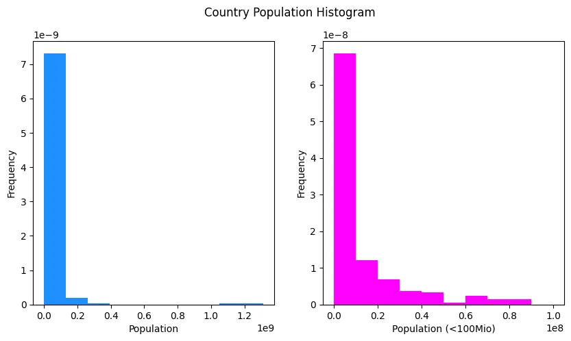
plt.figure(figsize=(12, 5))
plt.title('GDP ($ per capita) by Region')

sns.barplot(
    data=country_df,
    y='Region',
    x='GDP ($ per capita)',
    estimator=np.mean,
    errorbar='sd',
    orient='h',
    palette='cool'
)

plt.savefig('assets/Scikit_Learn_78.webp', bbox_inches='tight')

plt.figure(figsize=(10, 6))

sns.scatterplot(
    y='Phones (per 1000)',
    x='GDP ($ per capita)',
    data=country_df,
    hue='Region',
    palette='cool',
).set_title('GDP ($ per capita) vs. Phones (per 1000)')

plt.savefig('assets/Scikit_Learn_79.webp', bbox_inches='tight')

plt.figure(figsize=(10, 6))

sns.scatterplot(
    y='Literacy (%)',
    x='GDP ($ per capita)',
    data=country_df,
    hue='Region',
    palette='cool',
).set_title('GDP ($ per capita) vs. Literacy (%)')

plt.savefig('assets/Scikit_Learn_80.webp', bbox_inches='tight')

plt.figure(figsize=(20, 12), dpi=200)
plt.title('Correlation Heatmap CIA Country Dataset')

sns.heatmap(
    country_df.corr(numeric_only=True),
    linewidth=0.5,
    cmap='seismic',
    annot=True
)

plt.savefig('assets/Scikit_Learn_81.webp', bbox_inches='tight')

plt.figure(figsize=(20, 12), dpi=200)
sns.clustermap(
    country_df.corr(numeric_only=True),
    linewidth=0.5,
    cmap='seismic',
    annot=False,
    col_cluster=False
)

plt.savefig('assets/Scikit_Learn_82.webp', bbox_inches='tight')

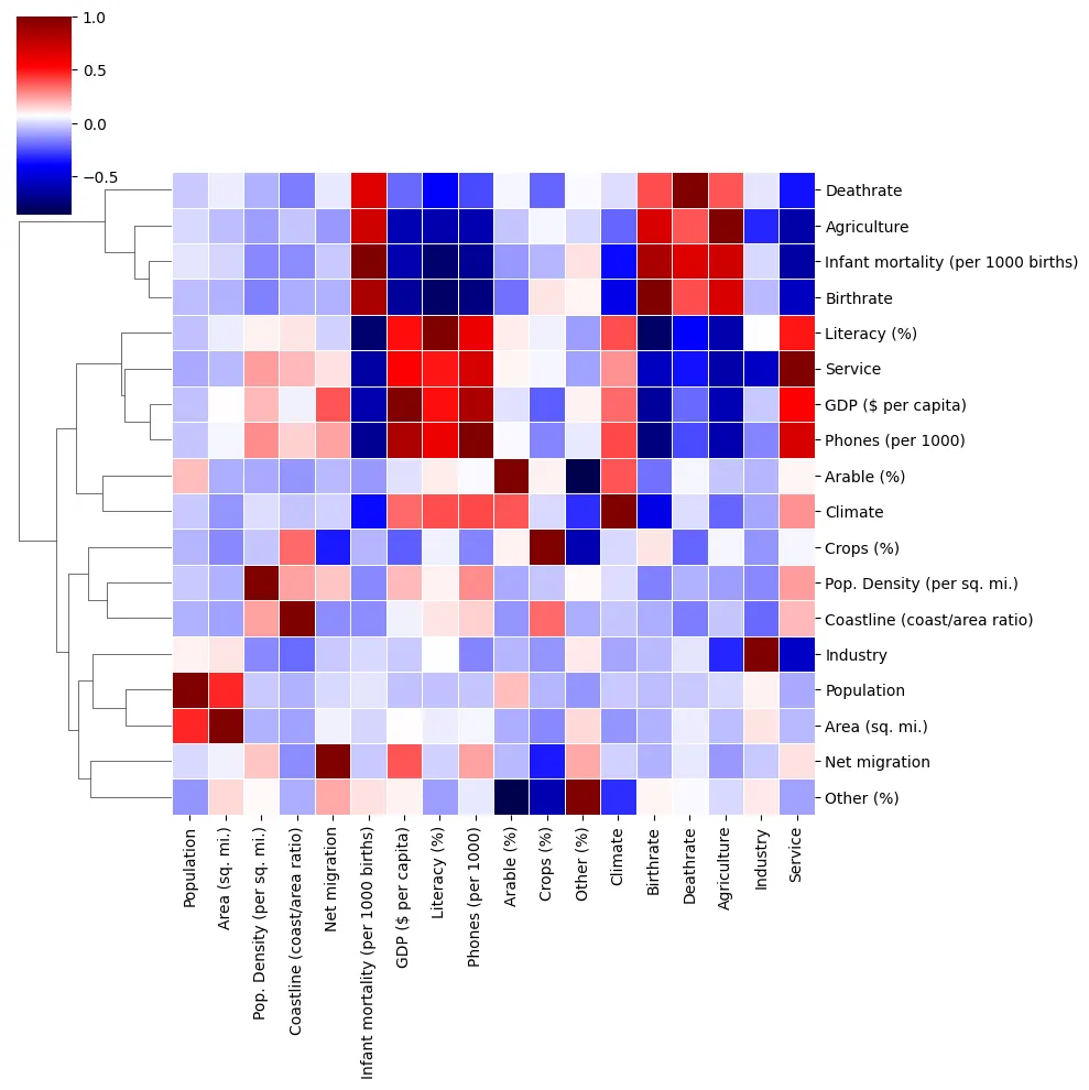
Dataset Preprocessing

# find columns with missing values
country_df.isnull().sum()

Country	0
Region	0
Population	0
Area (sq. mi.)	0
Pop. Density (per sq. mi.)	0
Coastline (coast/area ratio)	0
Net migration	3
Infant mortality (per 1000 births)	3
GDP ($ per capita)	1
Literacy (%)	18
Phones (per 1000)	4
Arable (%)	2
Crops (%)	2
Other (%)	2
Climate	22
Birthrate	3
Deathrate	4
Agriculture	15
Industry	16
Service	15
dtype: int64

# what countries don't have an agriculture value
country_df[pd.isnull(country_df['Agriculture'])]['Country']
# all countries without agriculture data will not have a
# whole lot of agriculture output. The same is true for 'Industry'
# and 'Service' These values can be set to zero:

3	American Samoa
4	Andorra
78	Gibraltar
80	Greenland
83	Guam
134	Mayotte
140	Montserrat
144	Nauru
153	N. Mariana Islands
171	Saint Helena
174	St Pierre & Miquelon
177	San Marino
208	Turks & Caicos Is
221	Wallis and Futuna
223	Western Sahara
Name: Country, dtype: object

# set missing values to zero for Agriculture, Industry and Service
# define what default values you want to fill
values = \{
    "Agriculture": 0,
    "Industry": 0,
    "Service": 0,
\}
# and replace missing with values
country_df = country_df.fillna(value=values)

# another datapoint that is often missing is climate
# the climate can be estimated by countries in the same Region
country_df[pd.isnull(country_df['Climate'])][['Country', 'Region', 'Climate']]

	Country	Region	Climate
5	Angola	SUB-SAHARAN AFRICA	NaN
36	Canada	NORTHERN AMERICA	NaN
50	Croatia	EASTERN EUROPE	NaN
66	Faroe Islands	WESTERN EUROPE	NaN
78	Gibraltar	WESTERN EUROPE	NaN
101	Italy	WESTERN EUROPE	NaN
115	Lebanon	NEAR EAST	NaN
118	Libya	NORTHERN AFRICA	NaN
120	Lithuania	BALTICS	NaN
121	Luxembourg	WESTERN EUROPE	NaN
129	Malta	WESTERN EUROPE	NaN
137	Moldova	C.W. OF IND. STATES	NaN
138	Monaco	WESTERN EUROPE	NaN
141	Morocco	NORTHERN AFRICA	NaN
145	Nepal	ASIA (EX. NEAR EAST)	NaN
169	Russia	C.W. OF IND. STATES	NaN
171	Saint Helena	SUB-SAHARAN AFRICA	NaN
174	St Pierre & Miquelon	NORTHERN AMERICA	NaN
177	San Marino	WESTERN EUROPE	NaN
181	Serbia	EASTERN EUROPE	NaN
186	Slovenia	EASTERN EUROPE	NaN
200	Tanzania	SUB-SAHARAN AFRICA	NaN

country_df[pd.isnull(country_df['Climate'])]['Region'].value_counts()

WESTERN EUROPE	7
SUB-SAHARAN AFRICA	3
EASTERN EUROPE	3
NORTHERN AMERICA	2
NORTHERN AFRICA	2
C.W. OF IND. STATES	2
NEAR EAST	1
BALTICS	1
ASIA (EX. NEAR EAST)	1
Name: Region, dtype: int64

# the Region value has annoying whitespaces that need to be stripped
country_df['Region'] = country_df['Region'].apply(lambda x: x.strip())

# climate zones in western europe
country_df[country_df['Region'] == 'WESTERN EUROPE']['Climate'].value_counts()

# climate zones in SUB-SAHARAN AFRICA
country_df[country_df['Region'] == 'SUB-SAHARAN AFRICA']['Climate'].value_counts()

# climate zones in EASTERN EUROPE
country_df[country_df['Region'] == 'EASTERN EUROPE']['Climate'].value_counts()

# climate zones in NORTHERN AMERICA
country_df[country_df['Region'] == 'NORTHERN AMERICA']['Climate'].value_counts()

# climate zones in NORTHERN AFRICA
country_df[country_df['Region'] == 'NORTHERN AFRICA']['Climate'].value_counts()

# climate zones in C.W. OF IND. STATES
country_df[country_df['Region'] == 'C.W. OF IND. STATES']['Climate'].value_counts()

# climate zones in NEAR EAST
country_df[country_df['Region'] == 'NEAR EAST']['Climate'].value_counts()

# climate zones in BALTICS
country_df[country_df['Region'] == 'BALTICS']['Climate'].value_counts()

# climate zones in ASIA (EX. NEAR EAST)
country_df[country_df['Region'] == 'ASIA (EX. NEAR EAST)']['Climate'].value_counts()

# we can either use the top value to fill missing climate data points
# or use a mean value:
country_df['Climate'] = country_df['Climate'].fillna(country_df.groupby('Region')['Climate'].transform('mean'))

# there are more missing values, e.g. literacy:
country_df[pd.isnull(country_df['Literacy (%)'])][['Country', 'Region', 'Literacy (%)']]

	Country	Region	Literacy (%)
25	Bosnia & Herzegovina	EASTERN EUROPE	NaN
66	Faroe Islands	WESTERN EUROPE	NaN
74	Gaza Strip	NEAR EAST	NaN
78	Gibraltar	WESTERN EUROPE	NaN
80	Greenland	NORTHERN AMERICA	NaN
85	Guernsey	WESTERN EUROPE	NaN
99	Isle of Man	WESTERN EUROPE	NaN
104	Jersey	WESTERN EUROPE	NaN
108	Kiribati	OCEANIA	NaN
123	Macedonia	EASTERN EUROPE	NaN
134	Mayotte	SUB-SAHARAN AFRICA	NaN
144	Nauru	OCEANIA	NaN
185	Slovakia	EASTERN EUROPE	NaN
187	Solomon Islands	OCEANIA	NaN
209	Tuvalu	OCEANIA	NaN
220	Virgin Islands	LATIN AMER. & CARIB	NaN
222	West Bank	NEAR EAST	NaN
223	Western Sahara	NORTHERN AFRICA	NaN

# here we can also fill with mean values:
country_df['Literacy (%)'] = country_df['Literacy (%)'].fillna(country_df.groupby('Region')['Literacy (%)'].transform('mean'))

# the remaining rows with missing values can be dropped for now
country_df = country_df.dropna(axis=0)
country_df.isnull().sum()

Country	0
Region	0
Population	0
Area (sq. mi.)	0
Pop. Density (per sq. mi.)	0
Coastline (coast/area ratio)	0
Net migration	0
Infant mortality (per 1000 births)	0
GDP ($ per capita)	0
Literacy (%)	0
Phones (per 1000)	0
Arable (%)	0
Crops (%)	0
Other (%)	0
Climate	0
Birthrate	0
Deathrate	0
Agriculture	0
Industry	0
Service	0
dtype: int64

# drop the country column as it is a unique
# classifier that will not help with clustering
country_df_dropped = country_df.drop(['Country'], axis=1)

# the region column is useful but needs to be encoded
country_df_dropped = pd.get_dummies(country_df_dropped)

country_df_dropped.head(5).transpose()

	0	1	2	3	4
Population	31056997.00	3581655.000	3.293009e+07	57794.00	71201.00
Area (sq. mi.)	647500.00	28748.000	2.381740e+06	199.00	468.00
Pop. Density (per sq. mi.)	48.00	124.600	1.380000e+01	290.40	152.10
Coastline (coast/area ratio)	0.00	1.260	4.000000e-02	58.29	0.00
Net migration	23.06	-4.930	-3.900000e-01	-20.71	6.60
Infant mortality (per 1000 births)	163.07	21.520	3.100000e+01	9.27	4.05
GDP ($ per capita)	700.00	4500.000	6.000000e+03	8000.00	19000.00
Literacy (%)	36.00	86.500	7.000000e+01	97.00	100.00
Phones (per 1000)	3.20	71.200	7.810000e+01	259.50	497.20
Arable (%)	12.13	21.090	3.220000e+00	10.00	2.22
Crops (%)	0.22	4.420	2.500000e-01	15.00	0.00
Other (%)	87.65	74.490	9.653000e+01	75.00	97.78
Climate	1.00	3.000	1.000000e+00	2.00	3.00
Birthrate	46.60	15.110	1.714000e+01	22.46	8.71
Deathrate	20.34	5.220	4.610000e+00	3.27	6.25
Agriculture	0.38	0.232	1.010000e-01	0.00	0.00
Industry	0.24	0.188	6.000000e-01	0.00	0.00
Service	0.38	0.579	2.980000e-01	0.00	0.00
Region_ASIA (EX. NEAR EAST)	1.00	0.000	0.000000e+00	0.00	0.00
Region_BALTICS	0.00	0.000	0.000000e+00	0.00	0.00
Region_C.W. OF IND. STATES	0.00	0.000	0.000000e+00	0.00	0.00
Region_EASTERN EUROPE	0.00	1.000	0.000000e+00	0.00	0.00
Region_LATIN AMER. & CARIB	0.00	0.000	0.000000e+00	0.00	0.00
Region_NEAR EAST	0.00	0.000	0.000000e+00	0.00	0.00
Region_NORTHERN AFRICA	0.00	0.000	1.000000e+00	0.00	0.00
Region_NORTHERN AMERICA	0.00	0.000	0.000000e+00	0.00	0.00
Region_OCEANIA	0.00	0.000	0.000000e+00	1.00	0.00
Region_SUB-SAHARAN AFRICA	0.00	0.000	0.000000e+00	0.00	0.00
Region_WESTERN EUROPE	0.00	0.000	0.000000e+00	0.00	1.00

# to be able to compare all datapoints they need to be normalized
country_scaler = StandardScaler()
country_df_scaled = country_scaler.fit_transform(country_df_dropped)

Model Training

# finding a good k-value for number of cluster
ssd_country = []

for k in range(2,30):
    model = KMeans(n_clusters=k, n_init='auto')
    model.fit(country_df_scaled)
    
    ssd_country.append(model.inertia_)

plt.figure(figsize=(10,5))
plt.title('SSD as a Function of Number of Cluster')
plt.plot(range(2,30), ssd_country, 'o--')

plt.savefig('assets/Scikit_Learn_83.webp', bbox_inches='tight')

plt.figure(figsize=(10,5))
plt.title('Difference in SSD as a Function of Number of Clusters')
pd.Series(ssd_country).diff().plot(kind='bar')

plt.savefig('assets/Scikit_Learn_84.webp', bbox_inches='tight')

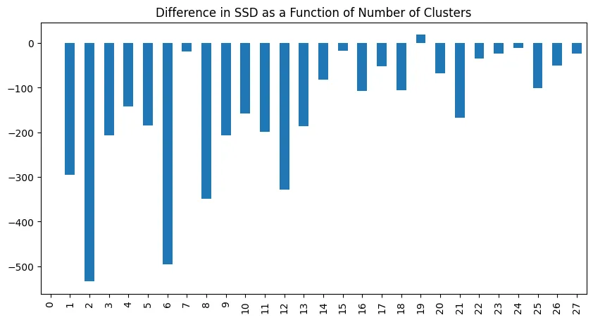
country_model = KMeans(
    n_clusters=14,
    n_init='auto',
    random_state=42
)
# fit to find cluster centers and predict what center every feature belongs to
country_cluster_labels = country_model.fit_predict(country_df_scaled)

Model Evaluation

# add predicted label to source dataframe
country_df['Cluster14'] = country_cluster_labels
country_df['Cluster14'].value_counts()

plt.figure(figsize=(10, 7))
sns.set(style='darkgrid')

# hue/style by categorical column
sns.scatterplot(
    x='GDP ($ per capita)',
    y='Literacy (%)',
    data=country_df,
    s=40,
    alpha=0.6,
    hue='Cluster14',
    palette='cool',
    style='Region'
).set_title('Country Clusters with k=14')

plt.savefig('assets/Scikit_Learn_85.webp', bbox_inches='tight')

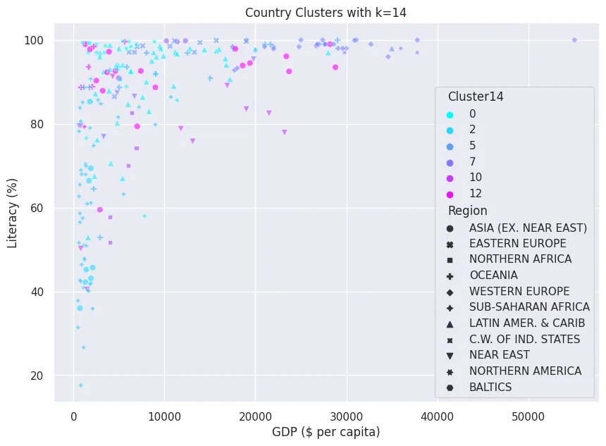
# repeat but only with 3 cluster
country_model2 = KMeans(
    n_clusters=3,
    n_init='auto',
    random_state=42
)
# fit to find cluster centers and predict what center every feature belongs to
country_cluster_labels2 = country_model2.fit_predict(country_df_scaled)

# add predicted label to source dataframe
country_df['Cluster3'] = country_cluster_labels2

plt.figure(figsize=(10, 7))
sns.set(style='darkgrid')

# hue/style by categorical column
sns.scatterplot(
    x='GDP ($ per capita)',
    y='Literacy (%)',
    data=country_df,
    s=40,
    alpha=0.6,
    hue='Cluster3',
    palette='cool',
    style='Region'
).set_title('Country Clusters with k=3')

plt.savefig('assets/Scikit_Learn_86.webp', bbox_inches='tight')

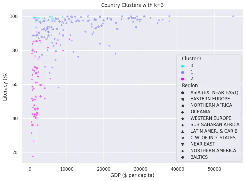
# How do the feature correlate with the predicted labels
country_label_corr = country_df.corr()['Cluster3']
print(country_label_corr.iloc[:-1].sort_values())

Feature Correlation

Literacy (%)	-0.413704
Crops (%)	-0.152936
Coastline (coast/area ratio)	-0.132610
Service	-0.070495
Area (sq. mi.)	-0.062183
Phones (per 1000)	-0.037538
Population	-0.024969
Industry	0.008487
Arable (%)	0.034891
Climate	0.049659
Other (%)	0.050444
Pop. Density (per sq. mi.)	0.101062
GDP ($ per capita)	0.122206
Agriculture	0.250750
Net migration	0.316226
Birthrate	0.369940
Infant mortality (per 1000 births)	0.412365
Deathrate	0.575814
Name: Cluster, dtype: float64

plt.figure(figsize=(10,6))
country_label_corr.iloc[:-1].sort_values().plot(kind='barh')
plt.title('Feature Importance')

plt.savefig('assets/Scikit_Learn_87.webp', bbox_inches='tight')

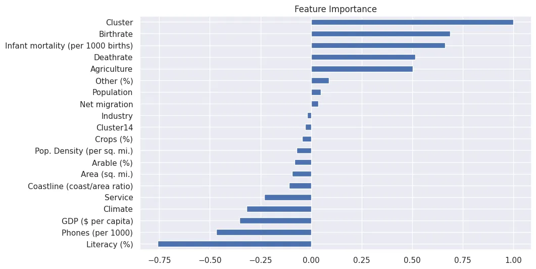
Plotly Choropleth Map

iso_codes = pd.read_csv('datasets/country-iso-codes.csv')
iso_map = iso_codes.set_index('Country')['ISO Code'].to_dict()

country_df['ISO Code'] = country_df['Country'].map(iso_map)
country_df[['Country','ISO Code']].head(5)

	Country	ISO Code
0	Afghanistan	AFG
1	Albania	ALB
2	Algeria	DZA
3	American Samoa	ASM
4	Andorra	AND

fig = px.choropleth(
    country_df,
    locations='ISO Code',
    color='Cluster3',
    hover_name='Country',
    color_continuous_scale=px.colors.sequential.Plasma
)

fig.show()

fig = px.choropleth(
    country_df,
    locations='ISO Code',
    color='Cluster14',
    hover_name='Country',
    color_continuous_scale=px.colors.sequential.Plasma
)

fig.show()

Unsupervised Learning - Agglomerative Clustering

Dataset Preprocessing

autompg_data: The Auto-MPG dataset for regression Revised from CMU StatLib library, data concerns city-cycle fuel consumption

autoMPG_df = pd.read_csv('datasets/auto-mpg.csv')
autoMPG_df.head(5)

	mpg	cylinders	displacement	horsepower	weight	acceleration	model_year	origin	name
0	18.0	8	307.0	130.0	3504	12.0	70	usa	chevrolet chevelle malibu
1	15.0	8	350.0	165.0	3693	11.5	70	usa	buick skylark 320
2	18.0	8	318.0	150.0	3436	11.0	70	usa	plymouth satellite
3	16.0	8	304.0	150.0	3433	12.0	70	usa	amc rebel sst
4	17.0	8	302.0	140.0	3449	10.5	70	usa	ford torino

autoMPG_df['origin'].value_counts()
# there are only 3 countries of origin - can be turned into a dummy variable

autoMPG_dummy_df = pd.get_dummies(autoMPG_df.drop('name', axis=1))
autoMPG_dummy_df.head(5)

	mpg	cylinders	displacement	horsepower	weight	acceleration	model_year	origin_europe	origin_japan	origin_usa
0	18.0	8	307.0	130.0	3504	12.0	70	False	False	True
1	15.0	8	350.0	165.0	3693	11.5	70	False	False	True
2	18.0	8	318.0	150.0	3436	11.0	70	False	False	True
3	16.0	8	304.0	150.0	3433	12.0	70	False	False	True
4	17.0	8	302.0	140.0	3449	10.5	70	False	False	True

# normalize dataset
scaler = MinMaxScaler()
autoMPG_scaled = pd.DataFrame(
    scaler.fit_transform(autoMPG_dummy_df), columns=autoMPG_dummy_df.columns
)
autoMPG_scaled.describe()

	mpg	cylinders	displacement	horsepower	weight	acceleration	model_year	origin_europe	origin_japan	origin_usa
count	392.000000	392.000000	392.000000	392.000000	392.000000	392.000000	392.000000	392.000000	392.000000	392.000000
mean	0.384200	0.494388	0.326646	0.317768	0.386897	0.448888	0.498299	0.173469	0.201531	0.625000
std	0.207580	0.341157	0.270398	0.209191	0.240829	0.164218	0.306978	0.379136	0.401656	0.484742
min	0.000000	0.000000	0.000000	0.000000	0.000000	0.000000	0.000000	0.000000	0.000000	0.000000
25%	0.212766	0.200000	0.095607	0.157609	0.173589	0.343750	0.250000	0.000000	0.000000	0.000000
50%	0.365691	0.200000	0.214470	0.258152	0.337539	0.446429	0.500000	0.000000	0.000000	1.000000
75%	0.531915	1.000000	0.536822	0.434783	0.567550	0.537202	0.750000	0.000000	0.000000	1.000000
max	1.000000	1.000000	1.000000	1.000000	1.000000	1.000000	1.000000	1.000000	1.000000	1.000000

plt.figure(figsize=(12,10))

sns.heatmap(autoMPG_scaled, annot=False, cmap='viridis')

plt.savefig('assets/Scikit_Learn_90.webp', bbox_inches='tight')

sns.clustermap(
    autoMPG_scaled.corr(numeric_only=True),
    linewidth=0.5,
    cmap='seismic',
    annot=True,
    col_cluster=False
)

plt.savefig('assets/Scikit_Learn_91.webp', bbox_inches='tight')

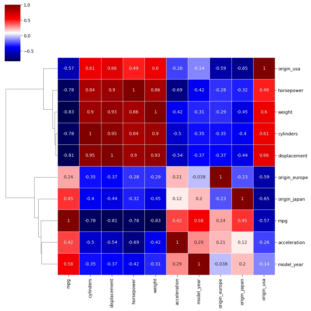
Assigning Cluster Labels

Known Number of Clusters

# there are ~ 4 clusters visible - let's try to agglomerate them
autoMPG_model = AgglomerativeClustering(n_clusters=4)
cluster_labels = autoMPG_model.fit_predict(autoMPG_scaled)
autoMPG_df['label'] = cluster_labels
autoMPG_df.head(5)

	mpg	cylinders	displacement	horsepower	weight	acceleration	model_year	origin	name	label
0	18.0	8	307.0	130.0	3504	12.0	70	usa	chevrolet chevelle malibu	2
1	15.0	8	350.0	165.0	3693	11.5	70	usa	buick skylark 320	2
2	18.0	8	318.0	150.0	3436	11.0	70	usa	plymouth satellite	2
3	16.0	8	304.0	150.0	3433	12.0	70	usa	amc rebel sst	2
4	17.0	8	302.0	140.0	3449	10.5	70	usa	ford torino	2

plt.figure(figsize=(12,5))
sns.scatterplot(
    x='mpg',
    y='horsepower',
    data=autoMPG_df,
    hue='label',
    palette='cool_r',
    style='origin'
).set_title('Horsepower as a function of Miles-per-gallon')

plt.savefig('assets/Scikit_Learn_92.webp', bbox_inches='tight')

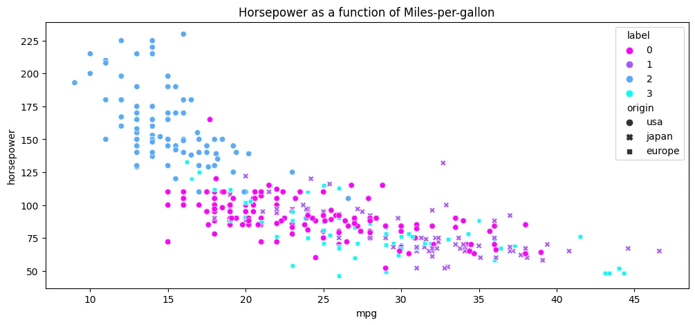
plt.figure(figsize=(12,5))
sns.scatterplot(
    x='model_year',
    y='mpg',
    data=autoMPG_df,
    hue='label',
    palette='cool_r',
    style='origin'
).set_title('Model Year as a function of Miles-per-gallon')
plt.legend(bbox_to_anchor=(1.01,1.01))

plt.savefig('assets/Scikit_Learn_93.webp', bbox_inches='tight')

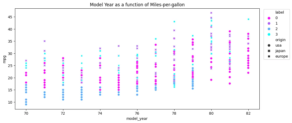
figure, axes = plt.subplots(1, 3, sharex=True,figsize=(15, 5))
figure.suptitle('Country of Origin')

axes[0].set_title('second chart with no data')

sns.scatterplot(
    x='horsepower',
    y='mpg',
    data=autoMPG_df[autoMPG_df['origin'] == 'europe'],
    hue='label',
    palette='cool_r',
    style='model_year',
    ax=axes[0]
).set_title('Europe')

axes[1].set_title('Europe')

sns.scatterplot(
    x='horsepower',
    y='mpg',
    data=autoMPG_df[autoMPG_df['origin'] == 'japan'],
    hue='label',
    palette='cool_r',
    style='model_year',
    ax=axes[1]
).set_title('Japan')

axes[2].set_title('second chart with no data')

sns.scatterplot(
    x='horsepower',
    y='mpg',
    data=autoMPG_df[autoMPG_df['origin'] == 'usa'],
    hue='label',
    palette='cool_r',
    style='model_year',
    ax=axes[2]
).set_title('USA') 
plt.legend(bbox_to_anchor=(1.01,1.01))

plt.savefig('assets/Scikit_Learn_94.webp', bbox_inches='tight')
# nice... perfect separation by country!

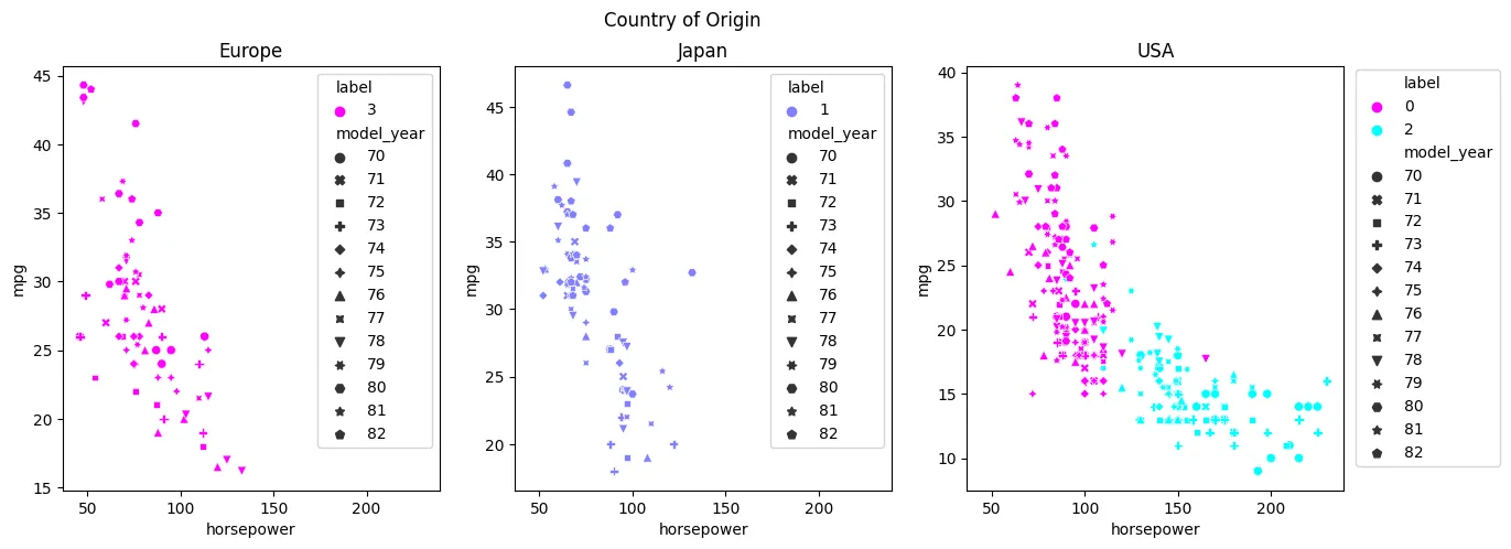
Unknown Number of Clusters

The Clustermap created above allowed us to estimate the amount of clusters needed to accuratly label the dataset based on the Dendrogram displayed on the left side. If we do not know how many clusters are present in our dataset we can define a maximum distance threshold a cluster can have before being merged with surrounding clusters. Setting this threshold to zero results in a number of clusters == number of datapoints.

autoMPG_model_auto = AgglomerativeClustering(
    n_clusters=None,
    metric='euclidean',
    distance_threshold=0
)
cluster_labels_auto = autoMPG_model_auto.fit_predict(autoMPG_scaled)
len(np.unique(cluster_labels_auto))
# threshold of zero leads to 392 clusters == number of rows in our dataset

# find out a good distance threshold
linkage_matrix = hierarchy.linkage(autoMPG_model_auto.children_)
linkage_matrix
# [`cluster[i]`, `cluster[j]`, `distance between`, `number of members`]

# to display this matrix we can use the above mentioned dendrogram
plt.figure(figsize=(20,10))
plt.title('Hierarchy Dendrogram for 8 Classes')
dendro = hierarchy.dendrogram(linkage_matrix, truncate_mode='lastp', p=9)

plt.savefig('assets/Scikit_Learn_95.webp', bbox_inches='tight')
# The higher the y-value the larger the distance between the connected clusters

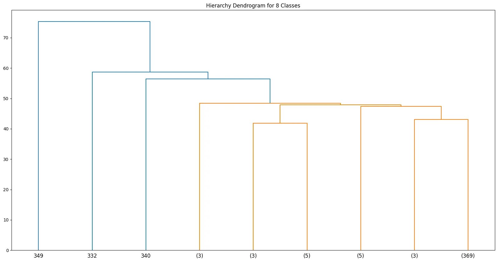
# since the miles-per-gallons are a good indicator for the label
# what is the max distance between two points here:
car_max_mpg = autoMPG_scaled.iloc[autoMPG_scaled['mpg'].idxmax()]
car_min_mpg = autoMPG_scaled.iloc[autoMPG_scaled['mpg'].idxmin()]

np.linalg.norm(car_max_mpg - car_min_mpg)
# 3.1128158766165406
# if the max distance is ~3 the threshold should be < 3

autoMPG_model_auto = AgglomerativeClustering(
    n_clusters=None,
    metric='euclidean',
    distance_threshold=2
)
cluster_labels_auto = autoMPG_model_auto.fit_predict(autoMPG_scaled)
len(np.unique(cluster_labels_auto))
# threshold of two leads to 11 clusters

autoMPG_model_auto = AgglomerativeClustering(
    n_clusters=None,
    metric='euclidean',
    distance_threshold=3
)
cluster_labels_auto = autoMPG_model_auto.fit_predict(autoMPG_scaled)
len(np.unique(cluster_labels_auto))
# threshold of three leads to 9 clusters

autoMPG_df['label_auto'] = cluster_labels_auto

figure, axes = plt.subplots(1, 3, sharex=True,figsize=(15, 6))
figure.suptitle('Country of Origin')

axes[0].set_title('second chart with no data')

sns.scatterplot(
    x='horsepower',
    y='mpg',
    data=autoMPG_df[autoMPG_df['origin'] == 'europe'],
    hue='label_auto',
    palette='cool_r',
    style='model_year',
    ax=axes[0]
).set_title('Europe')

axes[1].set_title('Europe')

sns.scatterplot(
    x='horsepower',
    y='mpg',
    data=autoMPG_df[autoMPG_df['origin'] == 'japan'],
    hue='label_auto',
    palette='cool_r',
    style='model_year',
    ax=axes[1]
).set_title('Japan')

axes[2].set_title('second chart with no data')

sns.scatterplot(
    x='horsepower',
    y='mpg',
    data=autoMPG_df[autoMPG_df['origin'] == 'usa'],
    hue='label_auto',
    palette='cool_r',
    style='model_year',
    ax=axes[2]
).set_title('USA') 
plt.legend(bbox_to_anchor=(1.01,1.01))

plt.savefig('assets/Scikit_Learn_96.webp', bbox_inches='tight')
# the division by countries is still there. but we are now getting
# sub-classes within each country - which might be important depending on your set goal

Unsupervised Learning - Density-based Spatial Clustering (DBSCAN)

DBSCAN vs KMeans

blobs_df = pd.read_csv('datasets/blobs.csv')
blobs_df.tail(2)

	X1	X2
1498	5.454552	6.461246
1499	-7.769230	7.014384

plt.figure(figsize=(12,5))
plt.title('Blobs Dataset')
sns.scatterplot(data=blobs_df, x='X1', y='X2')

plt.savefig('assets/Scikit_Learn_97.webp', bbox_inches='tight')

moons_df = pd.read_csv('datasets/moons.csv')
moons_df.tail(2)

	X1	X2
1498	1.803858	-0.154705
1499	0.203305	0.079049

plt.figure(figsize=(12,5))
plt.title('Moons Dataset')
sns.scatterplot(data=moons_df, x='X1', y='X2')

plt.savefig('assets/Scikit_Learn_98.webp', bbox_inches='tight')

circles_df = pd.read_csv('datasets/circles.csv')
circles_df.tail(2)

	X1	X2
1498	0.027432	-0.264891
1499	-0.216732	0.183006

plt.figure(figsize=(12,5))
plt.title('Circles Dataset')
sns.scatterplot(data=circles_df, x='X1', y='X2')

plt.savefig('assets/Scikit_Learn_99.webp', bbox_inches='tight')

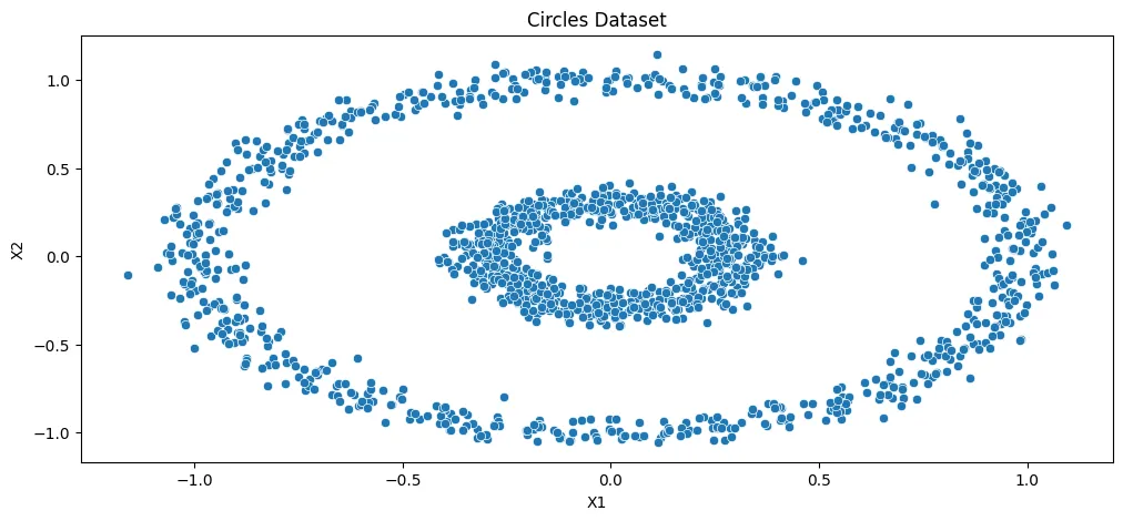
def display_categories(model, data, axis):
    labels = model.fit_predict(data)
    sns.scatterplot(data=data, x='X1', y='X2', hue=labels, palette='cool' , ax=axis)

km_model_blobs = KMeans(n_clusters=3, init='random', n_init='auto')
db_model_blobs = DBSCAN(eps=0.5, min_samples=5)

figure, axes = plt.subplots(1, 2, sharex=True,figsize=(12, 6))
figure.suptitle('3 Blobs Dataset')

axes[0].set_title('KMeans Clustering')
display_categories(km_model_blobs, blobs_df, axes[0])

axes[1].set_title('DBSCAN Clustering')
display_categories(db_model_blobs, blobs_df, axes[1])

plt.savefig('assets/Scikit_Learn_100.webp', bbox_inches='tight')

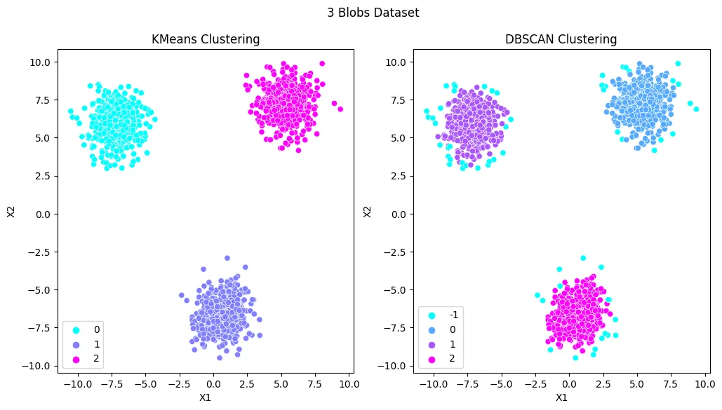
km_model_moons = KMeans(n_clusters=2, init='random', n_init='auto')
db_model_moons = DBSCAN(eps=0.2, min_samples=5)

figure, axes = plt.subplots(1, 2, sharex=True,figsize=(12, 6))
figure.suptitle('2 Moons Dataset')

axes[0].set_title('KMeans Clustering')
display_categories(km_model_moons, moons_df, axes[0])

axes[1].set_title('DBSCAN Clustering')
display_categories(db_model_moons, moons_df, axes[1])

plt.savefig('assets/Scikit_Learn_101.webp', bbox_inches='tight')

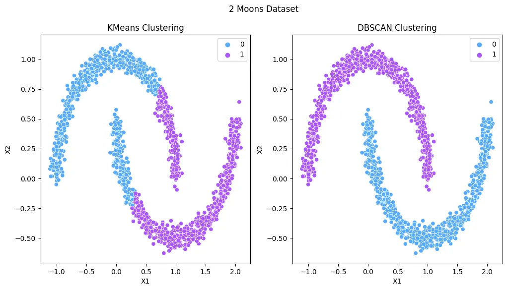
km_model_circles = KMeans(n_clusters=2, init='random', n_init='auto')
db_model_circles = DBSCAN(eps=0.2, min_samples=5)

figure, axes = plt.subplots(1, 2, sharex=True,figsize=(12, 6))
figure.suptitle('2 Circles Dataset')

axes[0].set_title('KMeans Clustering')
display_categories(km_model_circles, circles_df, axes[0])

axes[1].set_title('DBSCAN Clustering')
display_categories(db_model_circles, circles_df, axes[1])

plt.savefig('assets/Scikit_Learn_102.webp', bbox_inches='tight')

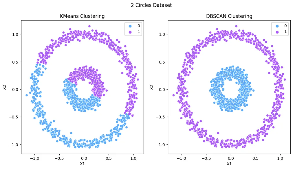
DBSCAN Hyperparameter Tuning

two_blobs_df = pd.read_csv('datasets/two-blobs.csv')
two_blobs_otl_df = pd.read_csv('datasets/two-blobs-outliers.csv')

# default hyperparameter
db_model_base = DBSCAN(eps=0.5, min_samples=5)

figure, axes = plt.subplots(1, 2, sharex=True,figsize=(12, 6))
figure.suptitle('2 Blobs Dataset - Default Hyperparameter')

axes[0].set_title('DBSCAN Clustering w/o Outliers')
display_categories(db_model_base, two_blobs_df, axes[0])

axes[1].set_title('DBSCAN Clustering with Outliers')
display_categories(db_model_base, two_blobs_otl_df, axes[1])

plt.savefig('assets/Scikit_Learn_103.webp', bbox_inches='tight')
# points around cluster 1 are assigned to be outliers

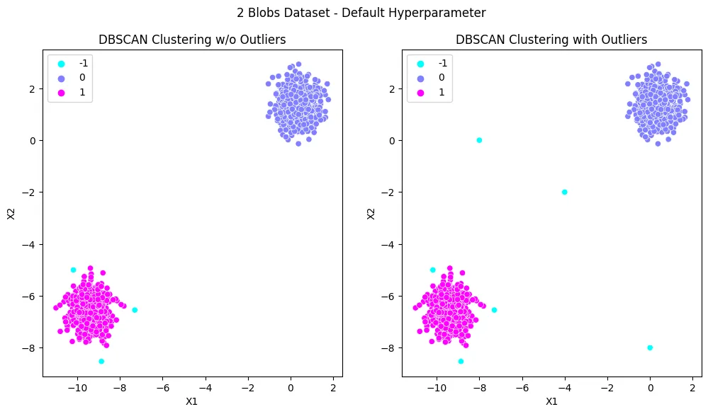
# reducing epsilon reduces the max distance (epsilon)
# points are allowed to have and still be assigned to a cluster
db_model_dec = DBSCAN(eps=0.001, min_samples=5)

figure, axes = plt.subplots(1, 2, sharex=True,figsize=(12, 6))
figure.suptitle('2 Blobs Dataset - Reduced Epsilon')

axes[0].set_title('DBSCAN Clustering w/o Outliers')
display_categories(db_model_dec, two_blobs_df, axes[0])

axes[1].set_title('DBSCAN Clustering with Outliers')
display_categories(db_model_dec, two_blobs_otl_df, axes[1])

plt.savefig('assets/Scikit_Learn_104.webp', bbox_inches='tight')
# distance is too small - every point becomes it's own cluster and is assigned as an outlier

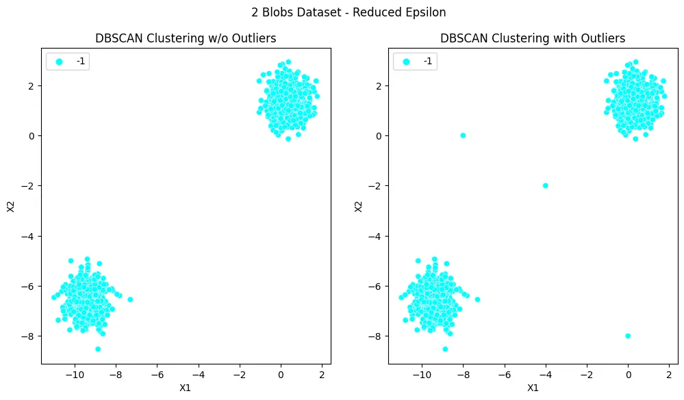
# increasing epsilon increases the max distance (epsilon)
# points are allowed to have and still be assigned to a cluster
db_model_inc = DBSCAN(eps=10, min_samples=5)

figure, axes = plt.subplots(1, 2, sharex=True,figsize=(12, 6))
figure.suptitle('2 Blobs Dataset - Increased Epsilon')

axes[0].set_title('DBSCAN Clustering w/o Outliers')
display_categories(db_model_inc, two_blobs_df, axes[0])

axes[1].set_title('DBSCAN Clustering with Outliers')
display_categories(db_model_inc, two_blobs_otl_df, axes[1])

plt.savefig('assets/Scikit_Learn_105.webp', bbox_inches='tight')
# distance is too big - every point becomes becomes part of the same cluster

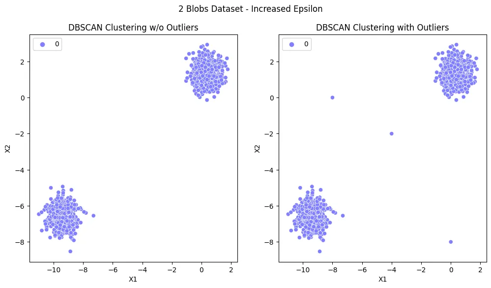
Elbow Plot

epsilon_value_range = np.linspace(0.0001, 1, 100)

n_outliers = []
perc_outlier = []
n_clusters = []

for epsilon in epsilon_value_range:
    dbscan_model = DBSCAN(eps=epsilon)
    dbscan_model.fit(two_blobs_otl_df)
    
    # total number of outliers
    n_outliers.append(np.sum(dbscan_model.labels_ == -1))
    # percentage of outliers
    perc_outlier.append(
        100 * np.sum(dbscan_model.labels_ == -1) / len(dbscan_model.labels_)
    )
    # number of clusters
    n_clusters.append(len(np.unique(dbscan_model.labels_)))

plt.figure(figsize=(12,5))
plt.title('Elbow Plot - DBSCAN Hyperparameter')
plt.xlabel('Epsilon (Max Distance between Points)')
plt.ylabel('Number of Outliers')
plt.ylim(0,10)
# we expect 3 outliers
plt.hlines(y=3, xmin=0, xmax=0.7, color='fuchsia')
# 3 outliers are reached somewhere around eps=0.7
plt.vlines(x=0.7, ymin=0, ymax=3, color='fuchsia')
sns.lineplot(x=epsilon_value_range, y=n_outliers)

plt.savefig('assets/Scikit_Learn_107.webp', bbox_inches='tight')

plt.figure(figsize=(12,5))
plt.title('Number of Clusters by Epsilon Range')
plt.xlabel('Epsilon (Max Distance between Points)')
plt.ylabel('Number of Clusters')
# we expect 2 clusters + outliers
plt.hlines(y=3, xmin=0, xmax=1, color='fuchsia')
plt.ylim(0,50)
plt.xlim(0,1)
sns.lineplot(x=epsilon_value_range, y=n_clusters)

plt.savefig('assets/Scikit_Learn_108.webp', bbox_inches='tight')
# we already reach 3 cluster with an epsilon of 0.2
# but as seen above we need an epsilon of 0.7 to reduce
# the number of outliers to 3

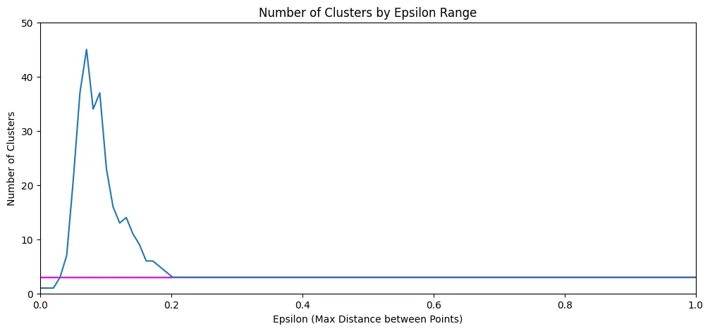
# find the optimum
# rule of thumb for min_samples = 2*n_dim
n_dim = two_blobs_otl_df.shape[1]
db_model_opt = DBSCAN(eps=0.7, min_samples=2*n_dim)

figure, axes = plt.subplots(1, 2, sharex=True,figsize=(12, 6))
figure.suptitle('2 Blobs Dataset - Optimal Epsilon')

axes[0].set_title('DBSCAN Clustering w/o Outliers')
display_categories(db_model_opt, two_blobs_df, axes[0])

axes[1].set_title('DBSCAN Clustering with Outliers')
display_categories(db_model_opt, two_blobs_otl_df, axes[1])

plt.savefig('assets/Scikit_Learn_106.webp', bbox_inches='tight')
# the 3 outliers are labled as such and every other point is assigned to one of the two clusters

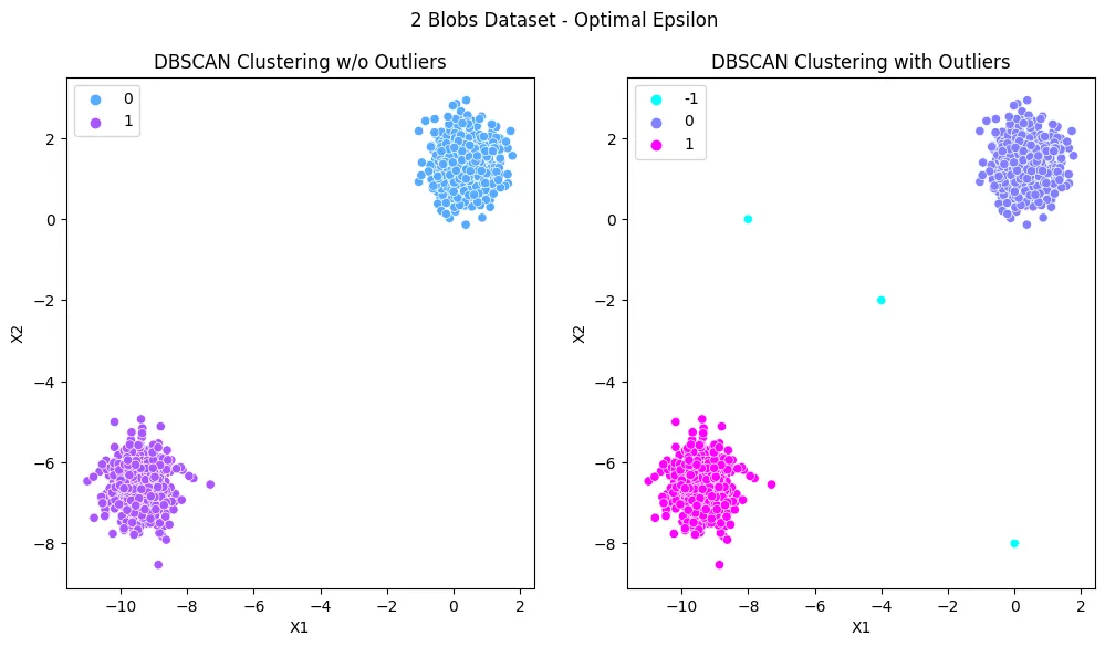
# find number of outliers
print('Number of Outliers', np.sum(db_model_opt.labels_ == -1))
# Number of Outliers 3
# get outlier percentage
print('Percentage of Outliers', (100 * np.sum(db_model_opt.labels_ == -1) / len(db_model_opt.labels_)).round(2),'%')
# Percentage of Outliers 0.3 %

Realworld Dataset

Wholesale customers The data set refers to clients of a wholesale distributor. It includes the annual spending in monetary units (m.u.) on diverse product categories

Additional Information

1. FRESH: annual spending (m.u.) on fresh products (Continuous)
2. MILK: annual spending (m.u.) on milk products (Continuous)
3. GROCERY: annual spending (m.u.) on grocery products (Continuous)
4. FROZEN: annual spending (m.u.) on frozen products (Continuous)
5. DETERGENTS_PAPER: annual spending (m.u.) on detergents and paper products (Continuous)
6. DELICATESSEN: annual spending (m.u.)on and delicatessen products (Continuous)
7. CHANNEL: customers Channel - Horeca (Hotel/Restaurant/Cafe) or Retail channel (Nominal)
8. REGION: customers Region - Lisnon, Oporto or Other (Nominal)

Dataset Exploration

wholesale_df = pd.read_csv('datasets/wholesome-customers-data.csv')
wholesale_df.head(5)

	Channel	Region	Fresh	Milk	Grocery	Frozen	Detergents_Paper	Delicassen
0	2	3	12669	9656	7561	214	2674	1338
1	2	3	7057	9810	9568	1762	3293	1776
2	2	3	6353	8808	7684	2405	3516	7844
3	1	3	13265	1196	4221	6404	507	1788
4	2	3	22615	5410	7198	3915	1777	5185

wholesale_df.info()

plt.figure(figsize=(12,5))
plt.title('Whole Sale: Milk Products vs Groceries')
sns.scatterplot(
    data=wholesale_df,
    x='Milk', y='Grocery',
    hue='Channel', style='Region',
    palette='winter'
)

plt.savefig('assets/Scikit_Learn_109.webp', bbox_inches='tight')

plt.figure(figsize=(10, 5))
plt.title('Whole Sale: Milk Products by Distribution Channel')

sns.histplot(
    data=wholesale_df,
    x='Milk',
    bins=50,
    hue='Channel',
    palette='winter',
    kde=True
)

plt.savefig('assets/Scikit_Learn_110.webp', bbox_inches='tight')

sns.clustermap(
    wholesale_df.corr(),
    linewidth=0.5,
    cmap='winter',
    annot=True,
    col_cluster=False
)

plt.savefig('assets/Scikit_Learn_111.webp', bbox_inches='tight')

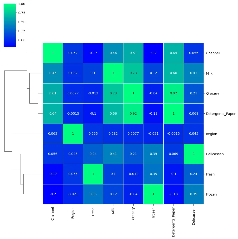
sns.pairplot(
    data=wholesale_df,
    hue='Region',
    palette='winter'
)

plt.savefig('assets/Scikit_Learn_112.webp', bbox_inches='tight')

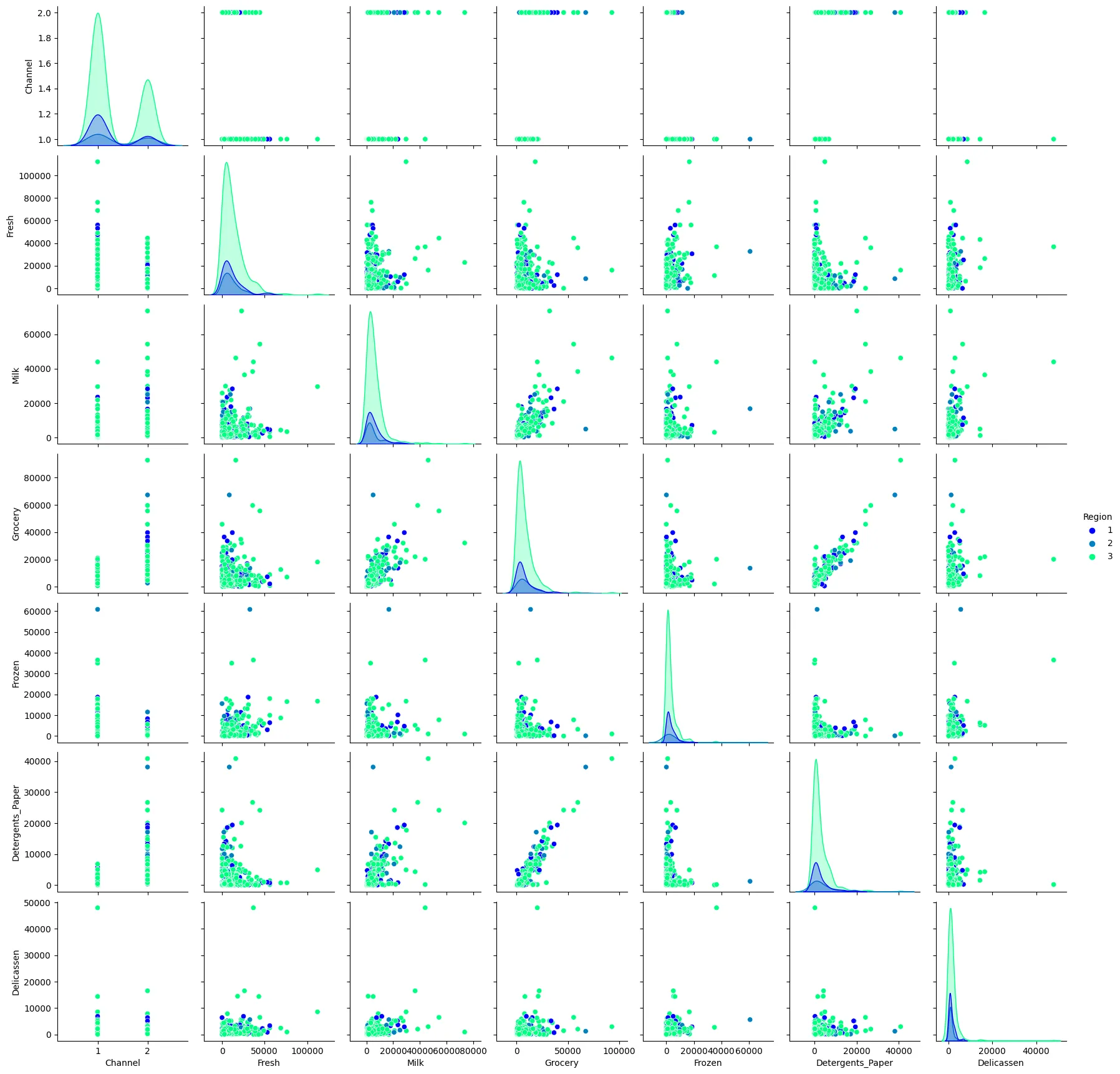
Data Preprocessing

# normalize feature set
scaler = StandardScaler()
wholesale_scaled = pd.DataFrame(
    scaler.fit_transform(wholesale_df), columns=wholesale_df.columns
)

wholesale_scaled.describe()

	Channel	Region	Fresh	Milk	Grocery	Frozen	Detergents_Paper	Delicassen
count	4.400000e+02	4.400000e+02	4.400000e+02	440.000000	4.400000e+02	4.400000e+02	4.400000e+02	4.400000e+02
mean	1.614870e-17	3.552714e-16	-3.431598e-17	0.000000	-4.037175e-17	3.633457e-17	2.422305e-17	-8.074349e-18
std	1.001138e+00	1.001138e+00	1.001138e+00	1.001138	1.001138e+00	1.001138e+00	1.001138e+00	1.001138e+00
min	-6.902971e-01	-1.995342e+00	-9.496831e-01	-0.778795	-8.373344e-01	-6.283430e-01	-6.044165e-01	-5.402644e-01
25%	-6.902971e-01	-7.023369e-01	-7.023339e-01	-0.578306	-6.108364e-01	-4.804306e-01	-5.511349e-01	-3.964005e-01
50%	-6.902971e-01	5.906683e-01	-2.767602e-01	-0.294258	-3.366684e-01	-3.188045e-01	-4.336004e-01	-1.985766e-01
75%	1.448652e+00	5.906683e-01	3.905226e-01	0.189092	2.849105e-01	9.946441e-02	2.184822e-01	1.048598e-01
max	1.448652e+00	5.906683e-01	7.927738e+00	9.183650	8.936528e+00	1.191900e+01	7.967672e+00	1.647845e+01

Model Hyperparameter Tuning

epsilon_value_range = np.linspace(0.001, 3, 100)
n_dim = wholesale_scaled.shape[1]

n_outliers = []
perc_outlier = []
n_clusters = []

for epsilon in epsilon_value_range:
    dbscan_model = DBSCAN(eps=epsilon, min_samples=2*n_dim)
    dbscan_model.fit(wholesale_scaled)
    
    # total number of outliers
    n_outliers.append(np.sum(dbscan_model.labels_ == -1))
    # percentage of outliers
    perc_outlier.append(
        100 * np.sum(dbscan_model.labels_ == -1) / len(dbscan_model.labels_)
    )
    # number of clusters
    n_clusters.append(len(np.unique(dbscan_model.labels_)))

plt.figure(figsize=(12,5))
plt.title('Elbow Plot - DBSCAN Hyperparameter')
plt.xlabel('Epsilon (Max Distance between Points)')
plt.ylabel('Number of Outliers')
plt.hlines(y=25, xmin=0, xmax=2, color='fuchsia')
plt.vlines(x=2, ymin=0, ymax=25, color='fuchsia')
sns.lineplot(x=epsilon_value_range, y=n_outliers)

plt.savefig('assets/Scikit_Learn_113.webp', bbox_inches='tight')

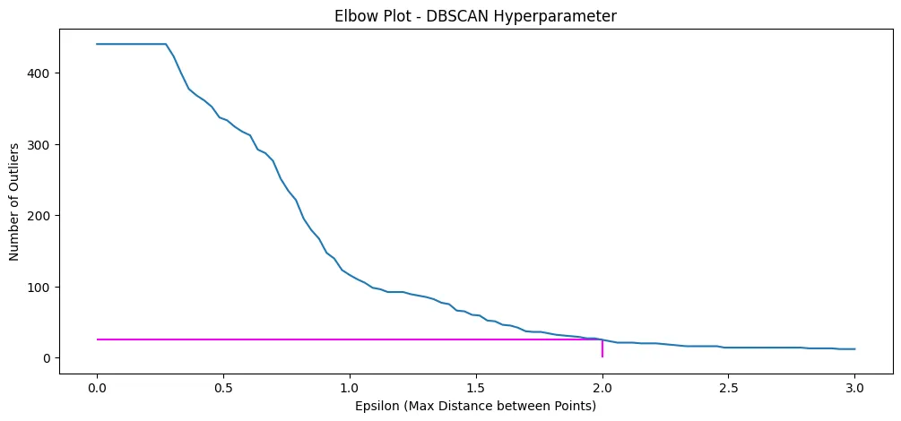
plt.figure(figsize=(12,5))
plt.title('Number of Clusters by Epsilon Range')
plt.xlabel('Epsilon (Max Distance between Points)')
plt.ylabel('Number of Clusters')
plt.hlines(y=3, xmin=0, xmax=2, color='fuchsia')
plt.vlines(x=2, ymin=0, ymax=3, color='fuchsia')
sns.lineplot(x=epsilon_value_range, y=n_clusters)

plt.savefig('assets/Scikit_Learn_114.webp', bbox_inches='tight')

def wholesale_categories(model, data, x, y, axis):
    labels = model.fit_predict(data)
    sns.scatterplot(data=data, x=x, y=y, hue=labels, palette='cool' , ax=axis)

db_model_opt = DBSCAN(eps=2.0, min_samples=2*n_dim)

figure, axes = plt.subplots(1, 2, sharex=True,figsize=(12, 6))
figure.suptitle('Whole Sale Dataset - DBSCAN Cluster (Normalized)')

axes[0].set_title('DBSCAN Clustering Milk Products vs Groceries')
wholesale_categories(
    model=db_model_opt,
    data=wholesale_scaled,
    x='Milk', y='Grocery',
    axis=axes[0]
)

axes[1].set_title('DBSCAN Clustering Milk Products vs Delicassen')
wholesale_categories(
    model=db_model_opt,
    data=wholesale_scaled,
    x='Milk', y='Delicassen',
    axis=axes[1]
)

plt.savefig('assets/Scikit_Learn_115a.webp', bbox_inches='tight')

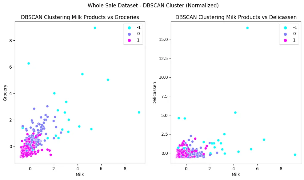
# add labels to original dataframe
wholesale_df['Label'] = db_model_opt.fit_predict(wholesale_scaled)
wholesale_df['Label'].head(5)

# remove outliers
wholesale_df_wo_otl = wholesale_df[wholesale_df['Label'] != -1]

db_model_opt = DBSCAN(eps=3.0, min_samples=2*n_dim)

figure, axes = plt.subplots(1, 2, sharex=True,figsize=(12, 6))
figure.suptitle('Whole Sale Dataset - DBSCAN Cluster (w/o Outliers)')

axes[0].set_title('DBSCAN Clustering Milk Products vs Groceries')
sns.scatterplot(
    data=wholesale_df_wo_otl,
    x='Milk', y='Grocery',
    hue='Label',
    palette='cool',
    ax=axes[0]
)

axes[1].set_title('DBSCAN Clustering Milk Products vs Delicassen')
sns.scatterplot(
    data=wholesale_df_wo_otl,
    x='Milk', y='Delicassen',
    hue='Label',
    palette='cool',
    ax=axes[1]
)

plt.savefig('assets/Scikit_Learn_115b.webp', bbox_inches='tight')

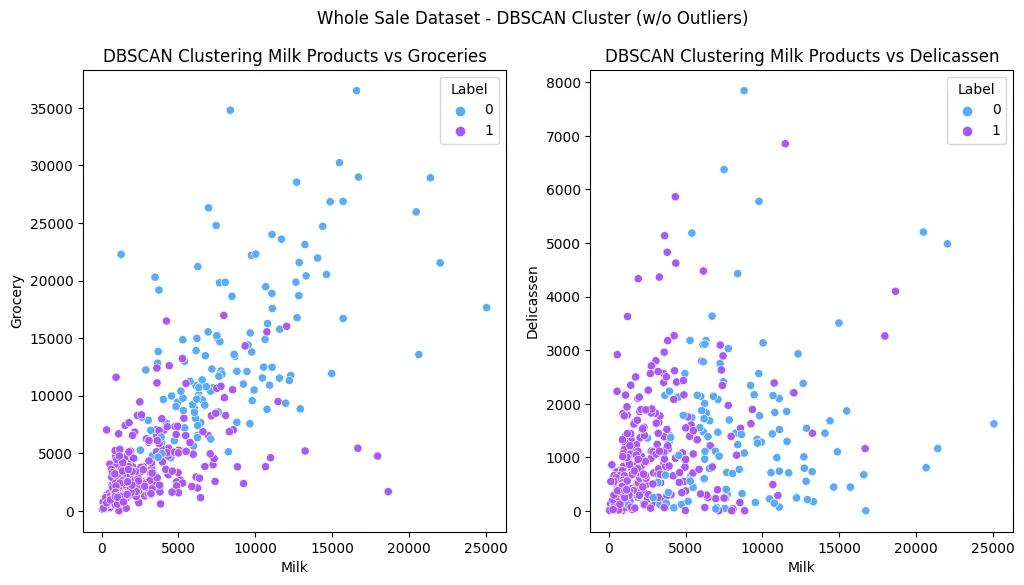
# see if the mean values of each cluster differ from each other
grouped_df = wholesale_df.groupby('Label').mean()

Label	Channel	Region	Fresh	Milk	Grocery	Frozen	Detergents_Paper	Delicassen
-1	1.52	2.480000	27729.920000	22966.960000	26609.600000	11289.640000	11173.560000	6707.160000
0	2.00	2.620155	8227.666667	8615.852713	13859.674419	1447.759690	5969.581395	1498.457364
1	1.00	2.513986	12326.972028	3023.559441	3655.328671	3086.181818	763.783217	1083.786713

scaler = MinMaxScaler()
grouped_scaler = pd.DataFrame(
    scaler.fit_transform(grouped_df), columns=grouped_df.columns, index=['Outlier', 'Cluster 1', 'Cluster 2']
)
grouped_scaler.head()

	Channel	Region	Fresh	Milk	Grocery	Frozen	Detergents_Paper	Delicassen
Outlier	0.52	0.000000	1.000000	1.000000	1.000000	1.000000	1.000000	1.000000
Cluster 1	1.00	1.000000	0.000000	0.280408	0.444551	0.000000	0.500087	0.073741
Cluster 2	0.00	0.242489	0.210196	0.000000	0.000000	0.166475	0.000000	0.000000

plt.figure(figsize=(12, 3))
plt.title('Scaled Cluster / Outliers Comparison (Normalized)')

sns.heatmap(
    grouped_scaler,
    linewidth=0.5,
    cmap='coolwarm',
    annot=True
)

plt.savefig('assets/Scikit_Learn_116.webp', bbox_inches='tight')

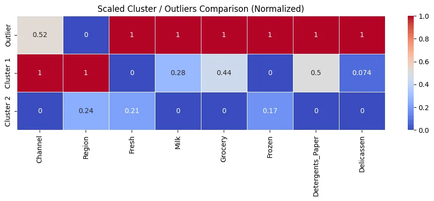
grouped_df = grouped_df.drop(['Labels'], axis=1)

# remove outlier
wholesale_clusters = grouped_df.drop(-1, axis=0)
wholesale_clusters.head()

Label	Channel	Region	Fresh	Milk	Grocery	Frozen	Detergents_Paper	Delicassen
0	2.0	2.620155	8227.666667	8615.852713	13859.674419	1447.759690	5969.581395	1498.457364
1	1.0	2.513986	12326.972028	3023.559441	3655.328671	3086.181818	763.783217	1083.786713

plt.figure(figsize=(12, 3))
plt.title('Mean Spending Values for Cluster 1 and 2')

sns.heatmap(
    wholesale_clusters,
    linewidth=0.5,
    cmap='coolwarm',
    annot=True
)

plt.savefig('assets/Scikit_Learn_117.webp', bbox_inches='tight')

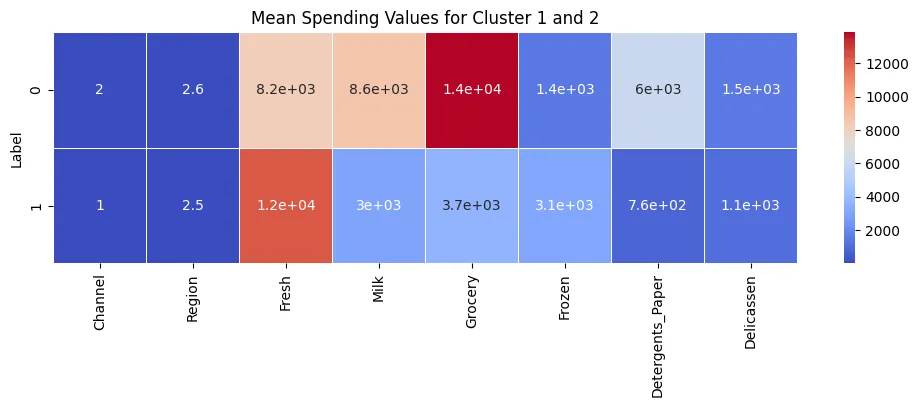
Dimensionality Reduction - Principal Component Analysis (PCA)

Dataset Preprocessing

Breast cancer wisconsin (diagnostic) dataset.

• Attribute Information:
  • radius (mean of distances from center to points on the perimeter)
  • texture (standard deviation of gray-scale values)
  • perimeter
  • area
  • smoothness (local variation in radius lengths)
  • compactness (perimeter^2 / area - 1.0)
  • concavity (severity of concave portions of the contour)
  • concave points (number of concave portions of the contour)
  • symmetry
  • fractal dimension ("coastline approximation" - 1)

The mean, standard error, and "worst" or largest (mean of the three worst/largest values) of these features were computed for each image, resulting in 30 features. For instance, field 0 is Mean Radius, field 10 is Radius SE, field 20 is Worst Radius.

• class:
  • WDBC-Malignant
  • WDBC-Benign

tumor_df = pd.read_csv('datasets/cancer-tumor-data-features.csv')
tumor_df.head(5).transpose()

	0	1	2	3	4
mean radius	17.990000	20.570000	19.690000	11.420000	20.290000
mean texture	10.380000	17.770000	21.250000	20.380000	14.340000
mean perimeter	122.800000	132.900000	130.000000	77.580000	135.100000
mean area	1001.000000	1326.000000	1203.000000	386.100000	1297.000000
mean smoothness	0.118400	0.084740	0.109600	0.142500	0.100300
mean compactness	0.277600	0.078640	0.159900	0.283900	0.132800
mean concavity	0.300100	0.086900	0.197400	0.241400	0.198000
mean concave points	0.147100	0.070170	0.127900	0.105200	0.104300
mean symmetry	0.241900	0.181200	0.206900	0.259700	0.180900
mean fractal dimension	0.078710	0.056670	0.059990	0.097440	0.058830
radius error	1.095000	0.543500	0.745600	0.495600	0.757200
texture error	0.905300	0.733900	0.786900	1.156000	0.781300
perimeter error	8.589000	3.398000	4.585000	3.445000	5.438000
area error	153.400000	74.080000	94.030000	27.230000	94.440000
smoothness error	0.006399	0.005225	0.006150	0.009110	0.011490
compactness error	0.049040	0.013080	0.040060	0.074580	0.024610
concavity error	0.053730	0.018600	0.038320	0.056610	0.056880
concave points error	0.015870	0.013400	0.020580	0.018670	0.018850
symmetry error	0.030030	0.013890	0.022500	0.059630	0.017560
fractal dimension error	0.006193	0.003532	0.004571	0.009208	0.005115
worst radius	25.380000	24.990000	23.570000	14.910000	22.540000
worst texture	17.330000	23.410000	25.530000	26.500000	16.670000
worst perimeter	184.600000	158.800000	152.500000	98.870000	152.200000
worst area	2019.000000	1956.000000	1709.000000	567.700000	1575.000000
worst smoothness	0.162200	0.123800	0.144400	0.209800	0.137400
worst compactness	0.665600	0.186600	0.424500	0.866300	0.205000
worst concavity	0.711900	0.241600	0.450400	0.686900	0.400000
worst concave points	0.265400	0.186000	0.243000	0.257500	0.162500
worst symmetry	0.460100	0.275000	0.361300	0.663800	0.236400
worst fractal dimension	0.118900	0.089020	0.087580	0.173000	0.076780

# normalizing data
scaler = StandardScaler()
tumor_scaled_arr = scaler.fit_transform(tumor_df)

tumor_scaled_df = pd.DataFrame(
    tumor_scaled_arr, columns=tumor_df.columns
)
tumor_scaled_df.head(5).transpose()

	0	1	2	3	4
mean radius	1.097064	1.829821	1.579888	-0.768909	1.750297
mean texture	-2.073335	-0.353632	0.456187	0.253732	-1.151816
mean perimeter	1.269934	1.685955	1.566503	-0.592687	1.776573
mean area	0.984375	1.908708	1.558884	-0.764464	1.826229
mean smoothness	1.568466	-0.826962	0.942210	3.283553	0.280372
mean compactness	3.283515	-0.487072	1.052926	3.402909	0.539340
mean concavity	2.652874	-0.023846	1.363478	1.915897	1.371011
mean concave points	2.532475	0.548144	2.037231	1.451707	1.428493
mean symmetry	2.217515	0.001392	0.939685	2.867383	-0.009560
mean fractal dimension	2.255747	-0.868652	-0.398008	4.910919	-0.562450
radius error	2.489734	0.499255	1.228676	0.326373	1.270543
texture error	-0.565265	-0.876244	-0.780083	-0.110409	-0.790244
perimeter error	2.833031	0.263327	0.850928	0.286593	1.273189
area error	2.487578	0.742402	1.181336	-0.288378	1.190357
smoothness error	-0.214002	-0.605351	-0.297005	0.689702	1.483067
compactness error	1.316862	-0.692926	0.814974	2.744280	-0.048520
concavity error	0.724026	-0.440780	0.213076	0.819518	0.828471
concave points error	0.660820	0.260162	1.424827	1.115007	1.144205
symmetry error	1.148757	-0.805450	0.237036	4.732680	-0.361092
fractal dimension error	0.907083	-0.099444	0.293559	2.047511	0.499328
worst radius	1.886690	1.805927	1.511870	-0.281464	1.298575
worst texture	-1.359293	-0.369203	-0.023974	0.133984	-1.466770
worst perimeter	2.303601	1.535126	1.347475	-0.249939	1.338539
worst area	2.001237	1.890489	1.456285	-0.550021	1.220724
worst smoothness	1.307686	-0.375612	0.527407	3.394275	0.220556
worst compactness	2.616665	-0.430444	1.082932	3.893397	-0.313395
worst concavity	2.109526	-0.146749	0.854974	1.989588	0.613179
worst concave points	2.296076	1.087084	1.955000	2.175786	0.729259
worst symmetry	2.750622	-0.243890	1.152255	6.046041	-0.868353
worst fractal dimension	1.937015	0.281190	0.201391	4.935010	-0.397100

Model Fitting

pca_model = PCA(n_components=2)
pca_results = pca_model.fit_transform(tumor_scaled_df)

print(pca_model.explained_variance_ratio_)
print(np.sum(pca_model.explained_variance_ratio_))
# the two principal components are able to describe
# 63% of the variance in the dataset
# [0.44272026 0.18971182]
# 0.6324320765155945

# adding components to original dataframe
tumor_df[['PC1','PC2']] = pca_results
tumor_df[['PC1','PC2']].head(5).transpose()

	0	1	2	3	4
PC1	9.192837	2.387802	5.733896	7.122953	3.935302
PC2	1.948583	-3.768172	-1.075174	10.275589	-1.948072

plt.figure(figsize=(12,5))
plt.title('Principal Component Analysis - Cancer Tumor Dataset')
sns.scatterplot(
    data=tumor_df,
    x='PC1', y='PC2'
)

plt.savefig('assets/Scikit_Learn_118.webp', bbox_inches='tight')

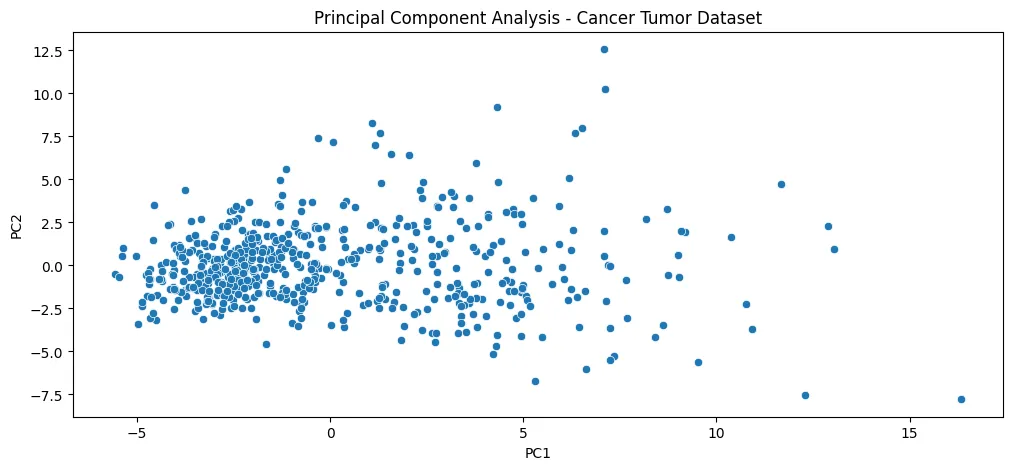
# get label data from dataset to confirm that we still have
# separably clusters after reducing the dimensions to 2
from sklearn.datasets import load_breast_cancer

tumor_dataset = load_breast_cancer()
tumor_dataset.keys()
# dict_keys(['data', 'target', 'frame', 'target_names', 'DESCR', 'feature_names', 'filename', 'data_module'])

tumor_dataset['target']

plt.figure(figsize=(12,5))
plt.title('PCA Cancer Tumor Dataset - Coloured by Labels')
sns.scatterplot(
    data=tumor_df,
    x='PC1', y='PC2',
    hue=tumor_dataset['target'],
    palette='winter'
)

plt.savefig('assets/Scikit_Learn_119.webp', bbox_inches='tight')

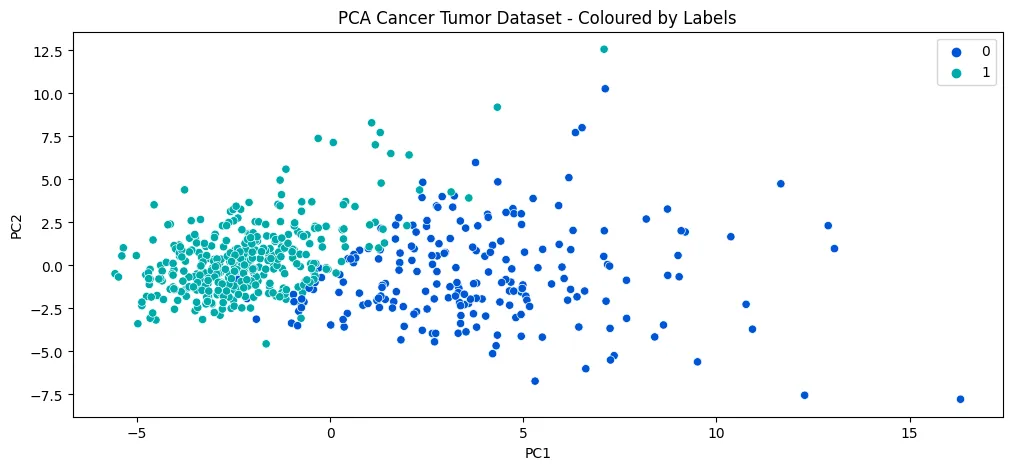
# as shown above we get around 63% of the variance explained by using 2 principal components
# since the dataset has 30 features 30 principal components will explain 100% of the variance

explained_variance = []

for n in range(1,31):
    pca = PCA(n_components=n)
    pca.fit(tumor_scaled_df)
    
    explained_variance.append(np.sum(pca.explained_variance_ratio_))

plt.figure(figsize=(10, 5))
plt.title('Explained Variance by Number of Principal Components')
plt.xlabel('Principal Components')
sns.set(style='darkgrid')
sns.barplot(
    data=pd.DataFrame(explained_variance, columns=['Explained Variance']),
    x=np.arange(1,31),
    y='Explained Variance'
)

plt.savefig('assets/Scikit_Learn_120.webp', bbox_inches='tight')

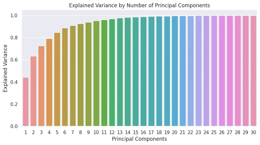
Dataset 2

• Digits Dataset

What handwritten numbers are the hardest to tell apart for a ML Model?

digits_df = pd.read_csv('datasets/digits.csv')
digits_df.head(5).transpose()

	0	1	2	3	4
pixel_0_0	0.0	0.0	0.0	0.0	0.0
pixel_0_1	0.0	0.0	0.0	0.0	0.0
pixel_0_2	5.0	0.0	0.0	7.0	0.0
pixel_0_3	13.0	12.0	4.0	15.0	1.0
pixel_0_4	9.0	13.0	15.0	13.0	11.0
...
pixel_7_4	10.0	16.0	11.0	13.0	16.0
pixel_7_5	0.0	10.0	16.0	9.0	4.0
pixel_7_6	0.0	0.0	9.0	0.0	0.0
pixel_7_7	0.0	0.0	0.0	0.0	0.0
number_label	0.0	1.0	2.0	3.0	4.0

# drop label column
X_digits = digits_df.drop('number_label', axis=1)
digits_labels = digits_df['number_label']

# select a single images
img_idx = 333
Single_Digit = np.array(X_digits.iloc[img_idx])
Single_Digit.shape
# the images inside the dataset are flattened
# (64,)

# need to be turned back into their 8x8 pixel format
Single_Digit = Single_Digit.reshape((8, 8))
Single_Digit.shape
# (8, 8)

# Display the Image
plt.figure(figsize=(4,4))
plt.imshow(Single_Digit, interpolation='nearest', cmap='plasma')
plt.title('Digit Label: %d' % digits_labels[img_idx])
plt.show()

plt.figure(figsize=(8,6))
plt.title('Digit Label: %d' % digits_labels[0])

sns.heatmap(
    Single_Digit,
    linewidth=0.5,
    cmap='plasma_r',
    annot=True
)

plt.savefig('assets/Scikit_Learn_122.webp', bbox_inches='tight')

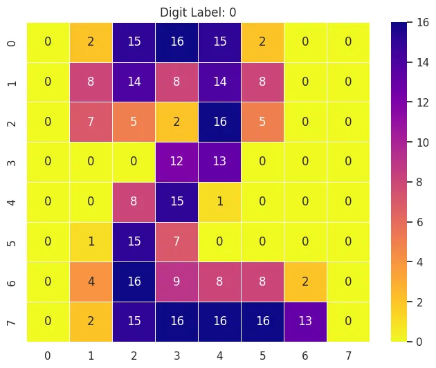
Dataset 2 Preprocessing

# normalize data
scaler = StandardScaler()
digits_scaled = pd.DataFrame(
    scaler.fit_transform(X_digits), columns=X_digits.columns
)
digits_scaled.head(5).transpose()

	0	1	2	3	4
pixel_0_0	0.000000	0.000000	0.000000	0.000000	0.000000
pixel_0_1	-0.335016	-0.335016	-0.335016	-0.335016	-0.335016
pixel_0_2	-0.043081	-1.094937	-1.094937	0.377661	-1.094937
pixel_0_3	0.274072	0.038648	-1.844742	0.744919	-2.551014
pixel_0_4	-0.664478	0.268751	0.735366	0.268751	-0.197863
...
pixel_7_3	0.208293	-0.249010	-2.078218	0.208293	-2.306869
pixel_7_4	-0.366771	0.849632	-0.164037	0.241430	0.849632
pixel_7_5	-1.146647	0.548561	1.565686	0.379040	-0.468564
pixel_7_6	-0.505670	-0.505670	1.695137	-0.505670	-0.505670
pixel_7_7	-0.196008	-0.196008	-0.196008	-0.196008	-0.196008

Model Fitting

pca_model2 = PCA(n_components=2)
pca_results2 = pca_model2.fit_transform(digits_scaled)
print(np.sum(pca_model2.explained_variance_ratio_))
# reducing the number of dimensions from 64 -> 2 leads to 22% explained variance

X_digits[['PC1','PC2']] = pca_results2
X_digits[['PC1','PC2']].head(5).transpose()

	0	1	2	3	4
PC1	1.914264	0.588997	1.302144	-3.020847	4.528854
PC2	-0.954564	0.924622	-0.317291	-0.868696	-1.093369

plt.figure(figsize=(12,5))
plt.title('PCA Digits Dataset - Coloured by Labels')
sns.scatterplot(
    data=X_digits,
    x='PC1', y='PC2',
    hue=digits_labels,
    palette='tab20'
)
plt.legend(bbox_to_anchor=(1.01,1.01))

plt.savefig('assets/Scikit_Learn_123.webp', bbox_inches='tight')
# numbers 4 and 7 are very distinct. There is some overlap between 6 and 0 and between 2 and 3
# but you can still get some separation. All the numbers in the middle are 'problematic' and 
# probably need a larger amount training data.

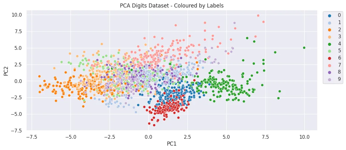
# how many components would we have to add to reach 80% explained variance
explained_variance = []

for n in range(1,65):
    pca = PCA(n_components=n)
    pca.fit(digits_scaled)
    
    explained_variance.append(np.sum(pca.explained_variance_ratio_))

plt.figure(figsize=(16, 5))
plt.title('Explained Variance by Number of Principal Components')
plt.xlabel('Principal Components')
sns.set(style='darkgrid')
sns.barplot(
    data=pd.DataFrame(explained_variance, columns=['Explained Variance']),
    x=np.arange(1,65),
    y='Explained Variance'
)

plt.savefig('assets/Scikit_Learn_124.webp', bbox_inches='tight')
# we need more than 20 principal components out of 64 to reach 80% expainable variance:

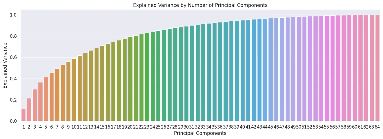
# rerun the training for 3 components for ~30% explained variance
pca_model3 = PCA(n_components=3)
pca_results3 = pca_model3.fit_transform(digits_scaled)
print(np.sum(pca_model3.explained_variance_ratio_))
# reducing the number of dimensions from 64 -> 3 leads to 30% explained variance

X_digits[['PC1','PC2','PC3']] = pca_results3
X_digits[['PC1','PC2','PC3']].head(5).transpose()

	0	1	2	3	4
PC1	1.914213	0.588981	1.302030	-3.020765	4.528946
PC2	-0.954510	0.924646	-0.317199	-0.868788	-1.093498
PC3	-3.945982	3.924713	3.023435	-0.801779	0.973213

%matplotlib notebook
fig = plt.figure(figsize=(8,8))
ax = plt.axes(projection='3d')
ax.scatter3D(
    xs=X_digits['PC1'],
    ys=X_digits['PC2'],
    zs=X_digits['PC3'],
    c=digits_labels,
    cmap='tab20'
)
ax.set_title('PCA Digits Dataset - Coloured by Labels')
ax.set(
    xticklabels=[],
    yticklabels=[],
    zticklabels=[],
    xlabel='PC1',
    ylabel='PC2',
    zlabel='PC3',
)

# plt.savefig('assets/Scikit_Learn_125.webp', bbox_inches='tight')