Introduction to Scikit-Image

Github Repository

• Introduction to Scikit-Image
  • Image Anatomy
    • Image Channels
    • Histogram
    • Image Transformations
  • Image Manipulation
    • Filtering Regional Maxima
    • Edges and Filters
    • Image Restoration
  • Image Segmentation
    • Feature Detection
    • Image Segmentation
    • Thresholding
    • Face Cascade Classifier

import numpy as np
from scipy import ndimage
from skimage import (
    data,
    io,
    color,
    exposure,
    transform,
    feature,
    measure,
    morphology,
    util,
    filters,
    img_as_float,
    restoration,
    segmentation,
    graph
)
import matplotlib.pyplot as plt
from matplotlib import patches

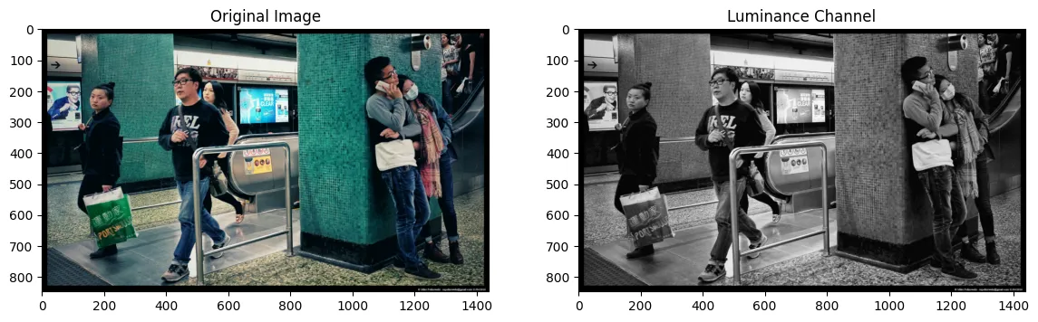
Image Anatomy

img = io.imread('assets/hk.jpg', as_gray=False)
img_gray = color.rgb2gray(img)
img.shape
# (847, 1440, 3)

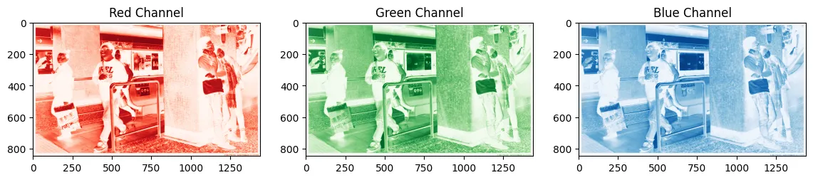
Image Channels

plt.figure(figsize=(14, 7))
plt.subplot(1, 2, 1)
plt.title("Original Image")
plt.imshow(img)
plt.subplot(1, 2, 2)
plt.title("Luminance Channel")
plt.imshow(img_gray, cmap='binary_r')

plt.savefig('assets/Scikit_Image_Intro_01.webp', bbox_inches='tight')

red = img[:,:,0]
green = img[:,:,1]
blue = img[:,:,2]

plt.figure(figsize=(14, 7))
plt.subplot(1, 3, 1)
plt.title("Red Channel")
plt.imshow(red, cmap='Reds')
plt.subplot(1, 3, 2)
plt.title("Green Channel")
plt.imshow(green, cmap='Greens')
plt.subplot(1, 3, 3)
plt.title("Blue Channel")
plt.imshow(blue, cmap='Blues')

plt.savefig('assets/Scikit_Image_Intro_02.webp', bbox_inches='tight')

Histogram

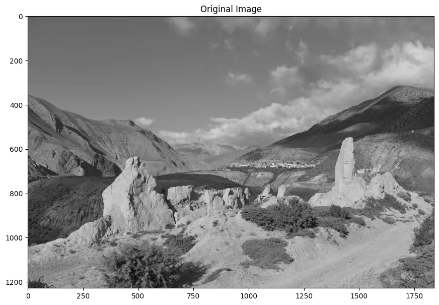
img2 = io.imread('assets/jomson.jpg', as_gray=True)

plt.figure(figsize=(14, 7))
plt.title("Original Image")
plt.imshow(img2, cmap='gray')

plt.savefig('assets/Scikit_Image_Intro_03.webp', bbox_inches='tight')

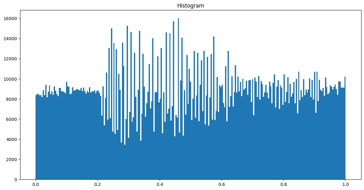
img_flat = img2.ravel()

plt.figure(figsize=(14, 7))
plt.title('Histogram')
plt.hist(img_flat, bins=255)

plt.savefig('assets/Scikit_Image_Intro_04.webp', bbox_inches='tight')

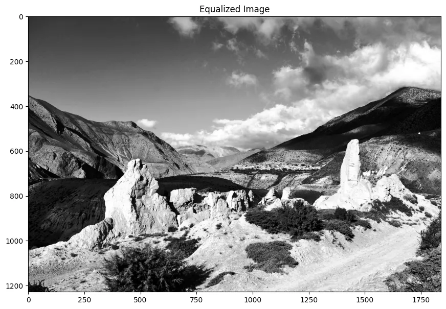
img_equalized = exposure.equalize_hist(img2)

img_flat2 = img_equalized.ravel()

plt.figure(figsize=(14, 7))
plt.title('Histogram')
plt.hist(img_flat2, bins=255)

plt.savefig('assets/Scikit_Image_Intro_05.webp', bbox_inches='tight')

plt.figure(figsize=(14, 7))
plt.title("Equalized Image")
plt.imshow(img_equalized, cmap='gray')

plt.savefig('assets/Scikit_Image_Intro_06.webp', bbox_inches='tight')

# match histograms
img_original = io.imread('assets/ice.jpg', as_gray=False)
hist_reference = io.imread('assets/ice2.jpg', as_gray=False)

img_matched = exposure.match_histograms(img_original, hist_reference, channel_axis=-1)

plt.figure(figsize=(14, 7))
plt.subplot(1, 3, 1)
plt.title("Original Image")
plt.imshow(img_original)
plt.subplot(1, 3, 2)
plt.title("Histogram Reference")
plt.imshow(hist_reference)
plt.subplot(1, 3, 3)
plt.title("Matched Image")
plt.imshow(img_matched)

plt.savefig('assets/Scikit_Image_Intro_09.webp', bbox_inches='tight')

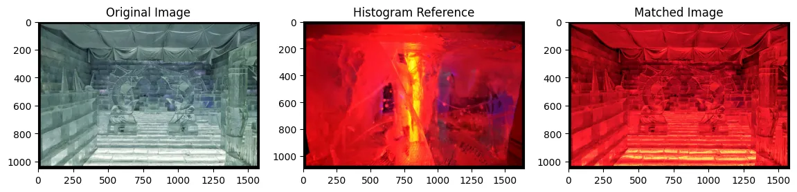
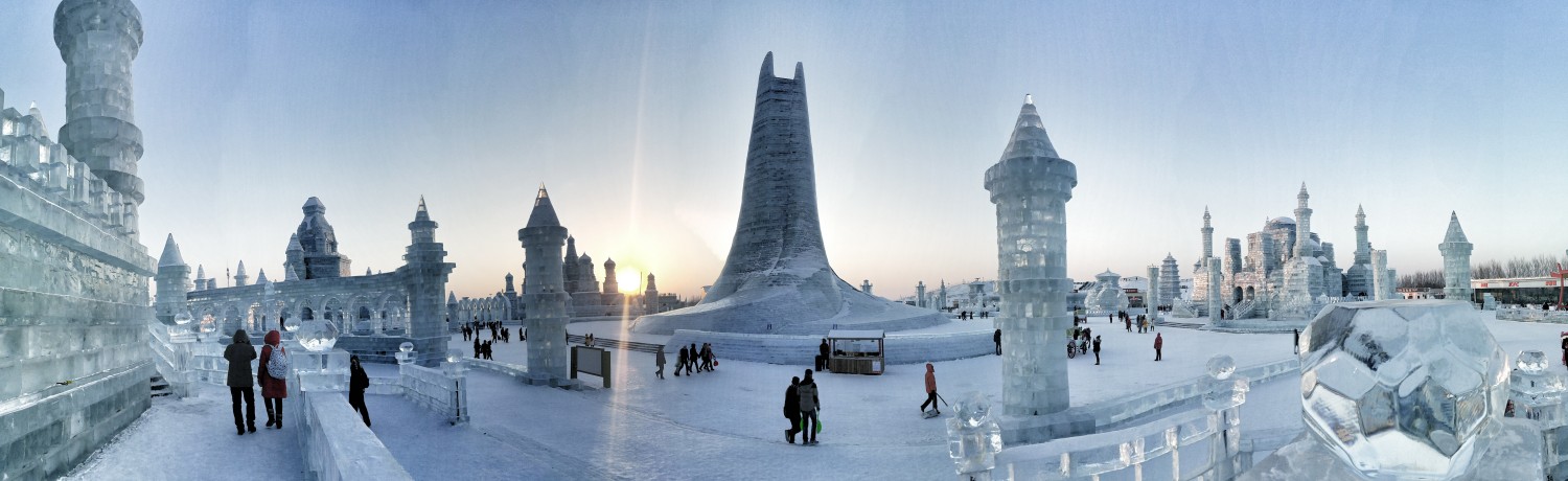
Image Transformations

img_ori.shape

img_ori = io.imread('assets/harbin.jpg', as_gray=False)

image_rescaled = transform.rescale(img_ori, 0.25, anti_aliasing=True)
img_thumb = transform.resize(img_ori, output_shape=(100, 157, 3), anti_aliasing=True)
img_swirled = transform.swirl(img_ori, radius=100, rotation=45)
img_rotated = transform.rotate(img_ori, angle=180)
img_downscaled = transform.downscale_local_mean(img_ori, factors=(4,3,3))
tform = transform.AffineTransform(
        shear=np.pi/6,
        )
img_warp = transform.warp(img_ori, tform.inverse)

plt.figure(figsize=(12, 8))
plt.subplot(2, 3, 1)
plt.title("rescale")
plt.imshow(image_rescaled)
plt.subplot(2, 3, 2)
plt.title("resize")
plt.imshow(img_thumb)
plt.subplot(2, 3, 3)
plt.title("swirl")
plt.imshow(img_swirled)
plt.subplot(2, 3, 4)
plt.title("rotate")
plt.imshow(img_rotated)
plt.subplot(2, 3, 5)
plt.title("resize_local_mean")
plt.imshow(img_downscaled)
plt.subplot(2, 3, 6)
plt.title("warp")
plt.imshow(img_warp)

plt.savefig('assets/Scikit_Image_Intro_07.webp', bbox_inches='tight')

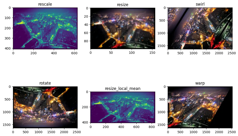
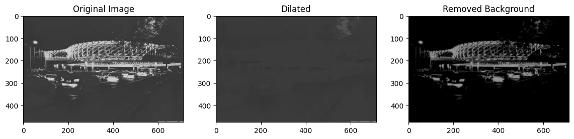
Image Manipulation

Filtering Regional Maxima

img_o = io.imread('assets/shenzhen.jpg', as_gray=False)

image = img_as_float(img_o)
image = ndimage.gaussian_filter(image, 1)

seed = np.copy(image)
seed[1:-1, 1:-1] = image.min()
mask = image

dilated = morphology.reconstruction(seed, mask, method='dilation')

plt.figure(figsize=(14, 7))
plt.subplot(1, 3, 1)
plt.title("Original Image")
plt.imshow(img_o, cmap='gray')
plt.subplot(1, 3, 2)
plt.title("Dilated")
plt.imshow(dilated, vmin=image.min(), vmax=image.max(), cmap='gray')
plt.subplot(1, 3, 3)
plt.title("Removed Background")
plt.imshow(image - dilated, cmap='gray')

plt.savefig('assets/Scikit_Image_Intro_10.webp', bbox_inches='tight')

Edges and Filters

img3 = io.imread('assets/ice_festival.jpg', as_gray=True)

# canny edge detector
img_edges1 = feature.canny(img3)
img_edges2 = feature.canny(img3, sigma=3)

# invert image
img_invert = util.invert(img3)
# perform skeletonization
img_skeleton = morphology.skeletonize(img_invert)

img_edge_roberts = filters.roberts(img3)
img_edge_sobel = filters.sobel(img3)

plt.figure(figsize=(12, 8))
plt.subplot(2, 3, 1)
plt.title("canny")
plt.imshow(img_edges1)
plt.subplot(2, 3, 2)
plt.title("canny sigma=3")
plt.imshow(img_edges2)
plt.subplot(2, 3, 3)
plt.title("invert")
plt.imshow(img_invert)
plt.subplot(2, 3, 4)
plt.title("skeletonize")
plt.imshow(img_skeleton)
plt.subplot(2, 3, 5)
plt.title("filters.roberts")
plt.imshow(img_edge_roberts)
plt.subplot(2, 3, 6)
plt.title("filters.sobel")
plt.imshow(img_edge_sobel)

plt.savefig('assets/Scikit_Image_Intro_08.webp', bbox_inches='tight')

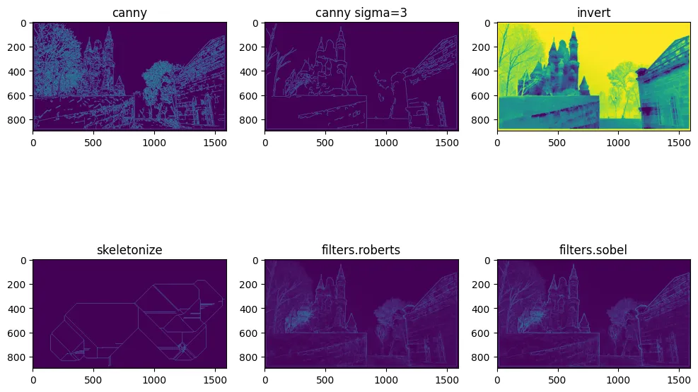
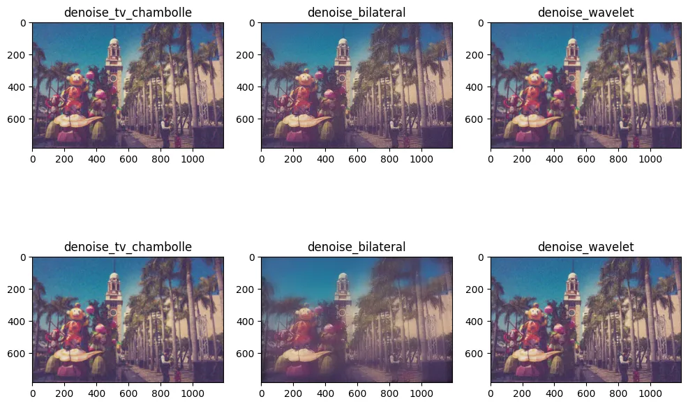
Image Restoration

img_o = io.imread('assets/tst.jpg', as_gray=False)
original = img_as_float(img_o)

sigma = 0.155
noisy = util.random_noise(original, var=sigma**2)
# Estimate the average noise standard deviation across color channels.
sigma_est = restoration.estimate_sigma(noisy, channel_axis=-1, average_sigmas=True)
# Due to clipping in random_noise, the estimate will be a bit smaller than the
# specified sigma.
print(f'Estimated Gaussian noise standard deviation = {sigma_est}')
# Estimated Gaussian noise standard deviation = 0.15293012739259768

# light
img_tv_chambolle = restoration.denoise_tv_chambolle(noisy, weight=0.1, channel_axis=-1)
img_bilateral = restoration.denoise_bilateral(noisy, sigma_color=0.05, sigma_spatial=15, channel_axis=-1)
img_wavelet = restoration.denoise_wavelet(noisy, channel_axis=-1, rescale_sigma=True)
# strong
img_tv_chambolle2 = restoration.denoise_tv_chambolle(noisy, weight=0.2, channel_axis=-1)
img_bilateral2 = restoration.denoise_bilateral(noisy, sigma_color=0.1, sigma_spatial=15, channel_axis=-1)
img_wavelet2 = restoration.denoise_wavelet(noisy, channel_axis=-1, convert2ycbcr=True, rescale_sigma=True)

plt.figure(figsize=(12, 8))
plt.subplot(2, 3, 1)
plt.title("denoise_tv_chambolle")
plt.imshow(img_tv_chambolle)
plt.subplot(2, 3, 2)
plt.title("denoise_bilateral")
plt.imshow(img_bilateral)
plt.subplot(2, 3, 3)
plt.title("denoise_wavelet")
plt.imshow(img_wavelet)
plt.subplot(2, 3, 4)
plt.title("denoise_tv_chambolle")
plt.imshow(img_tv_chambolle2)
plt.subplot(2, 3, 5)
plt.title("denoise_bilateral")
plt.imshow(img_bilateral2)
plt.subplot(2, 3, 6)
plt.title("denoise_wavelet")
plt.imshow(img_wavelet2)

plt.savefig('assets/Scikit_Image_Intro_11.webp', bbox_inches='tight')

img_o = io.imread('assets/ice3.jpg', as_gray=False)
original = img_as_float(img_o)

sigma = 0.1
noisy = util.random_noise(original, var=sigma**2)
# estimate the noise standard deviation from the noisy image
sigma_est = np.mean(restoration.estimate_sigma(original, channel_axis=-1))
print(f'estimated noise standard deviation = {sigma_est}')
# estimated noise standard deviation = 0.0017108497570321312

patch_kw = dict(patch_size=7,      # 5x5 patches
                patch_distance=11,  # 13x13 search area
                channel_axis=-1)
# slow algorithm
denoise_auto = restoration.denoise_nl_means(noisy, fast_mode=False,**patch_kw)
# slow algorithm, sigma provided
denoise = restoration.denoise_nl_means(noisy, h=1.15, sigma=sigma_est, fast_mode=False, **patch_kw)
# fast algorithm, sigma provided
denoise_fast = restoration.denoise_nl_means(noisy, h=0.1, sigma=sigma_est, fast_mode=True, **patch_kw)

plt.figure(figsize=(20, 10))
plt.subplot(2, 2, 1)
plt.title("Original")
plt.imshow(img_o)
plt.subplot(2, 2, 2)
plt.title("Noisy")
plt.imshow(noisy)
plt.subplot(2, 2, 3)
plt.title("Denoise Auto")
plt.imshow(denoise_auto)
plt.subplot(2, 2, 4)
plt.title("Denoise Fast")
plt.imshow(denoise_fast)

plt.savefig('assets/Scikit_Image_Intro_12.webp', bbox_inches='tight')

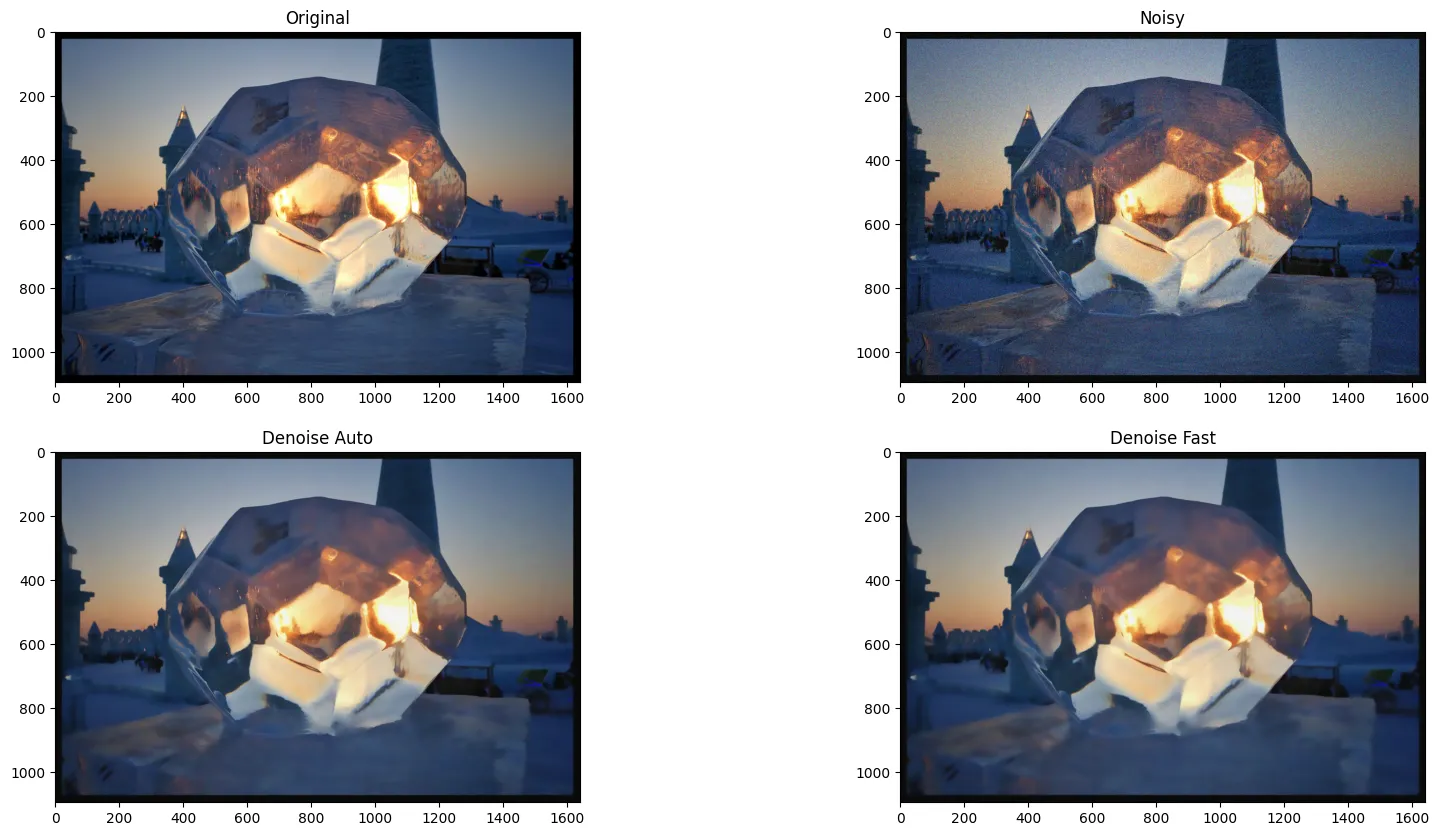
Image Segmentation

Feature Detection

img_o = io.imread('assets/abashiri.jpg', as_gray=True)
tform = transform.AffineTransform(scale=(0.5, 0.5), rotation=0.3,
                                  translation=(100, -25))
img_warp = transform.warp(img_o, tform)

detector = feature.CENSURE()
detector.detect(img_o)

fig, ax = plt.subplots(nrows=1, ncols=2, figsize=(12, 6))

ax[0].imshow(img_o, cmap=plt.cm.gray)
ax[0].scatter(detector.keypoints[:, 1], detector.keypoints[:, 0],
              2 ** detector.scales, facecolors='none', edgecolors='r')
ax[0].set_title("Original Image")

detector.detect(img_warp)

ax[1].imshow(img_warp, cmap=plt.cm.gray)
ax[1].scatter(detector.keypoints[:, 1], detector.keypoints[:, 0],
              2 ** detector.scales, facecolors='none', edgecolors='r')
ax[1].set_title('Transformed Image')

for a in ax:
    a.axis('off')

plt.savefig('assets/Scikit_Image_Intro_13.webp', bbox_inches='tight')

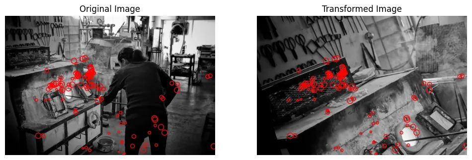
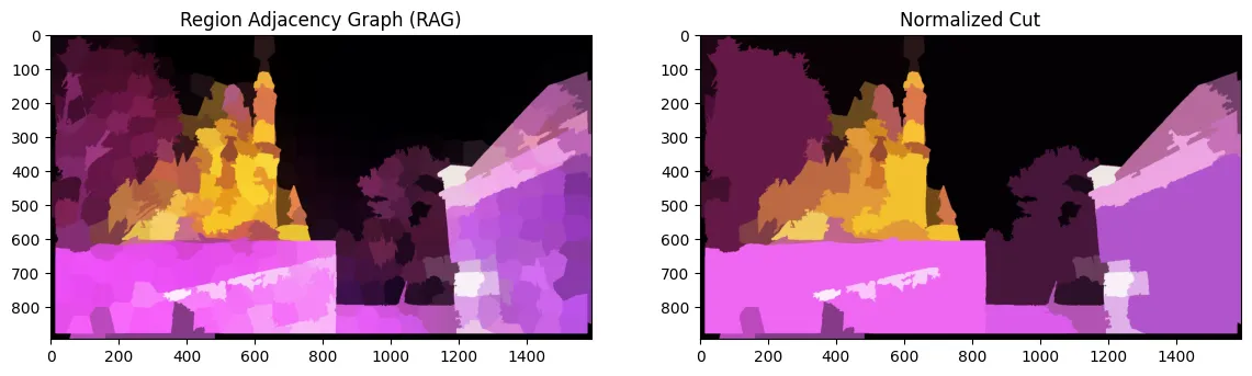
Image Segmentation

img3 = io.imread('assets/ice_festival.jpg', as_gray=False)

labels1 = segmentation.slic(img3, compactness=30, n_segments=400,start_label=1)
out1 = color.label2rgb(labels1, img3, kind='avg', bg_label=0)

g = graph.rag_mean_color(img3, labels1, mode='similarity')

labels2 = graph.cut_normalized(labels1, g)
out2 = color.label2rgb(labels2, img3, kind='avg', bg_label=0)

plt.figure(figsize=(14, 7))
plt.subplot(1, 2, 1)
plt.title("Region Adjacency Graph (RAG)")
plt.imshow(out1)
plt.subplot(1, 2, 2)
plt.title("Normalized Cut")
plt.imshow(out2)

plt.savefig('assets/Scikit_Image_Intro_14.webp', bbox_inches='tight')

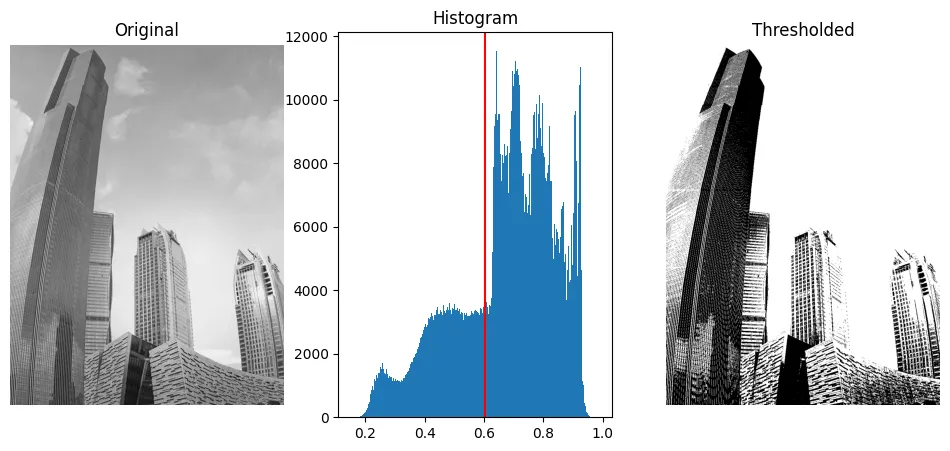
Thresholding

image = io.imread('assets/guangzhou.jpg', as_gray=True)
thresh = filters.threshold_otsu(image)
binary = image > thresh

fig, axes = plt.subplots(ncols=3, figsize=(12, 5))
ax = axes.ravel()
ax[0] = plt.subplot(1, 3, 1)
ax[1] = plt.subplot(1, 3, 2)
ax[2] = plt.subplot(1, 3, 3, sharex=ax[0], sharey=ax[0])

ax[0].imshow(image, cmap=plt.cm.gray)
ax[0].set_title('Original')
ax[0].axis('off')

ax[1].hist(image.ravel(), bins=256)
ax[1].set_title('Histogram')
ax[1].axvline(thresh, color='r')

ax[2].imshow(binary, cmap=plt.cm.gray)
ax[2].set_title('Thresholded')
ax[2].axis('off')

plt.savefig('assets/Scikit_Image_Intro_15.webp', bbox_inches='tight')

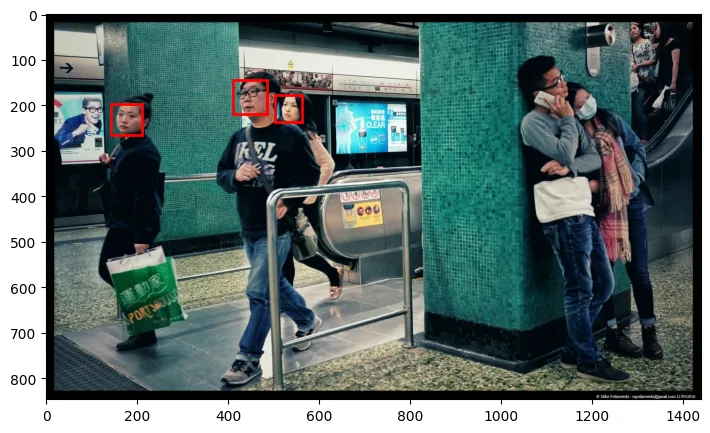
Face Cascade Classifier

# detection framework will also work with xml files from OpenCV.
!wget https://github.com/opencv/opencv/raw/master/data/lbpcascades/lbpcascade_frontalcatface.xml -P models

img = io.imread('assets/hk.jpg', as_gray=False)
# load the trained file from the module root.
frontal_face_cascade = data.lbp_frontal_face_cascade_filename()
# initialize the detector cascade.
detector = feature.Cascade(frontal_face_cascade)

detected = detector.detect_multi_scale(img=img,
                                       scale_factor=1.2,
                                       step_ratio=1,
                                       min_size=(60, 60),
                                       max_size=(123, 123))

plt.figure(figsize=(12, 5))
plt.imshow(img)
img_desc = plt.gca()
plt.set_cmap('gray')

for patch in detected:

    img_desc.add_patch(
        patches.Rectangle(
            (patch['c'], patch['r']),
            patch['width'],
            patch['height'],
            fill=False,
            color='r',
            linewidth=2
        )
    )

plt.savefig('assets/Scikit_Image_Intro_16.webp', bbox_inches='tight')