Harbin, China

OpenCV & SciPy and Scikit Image Cheat Sheet

OpenCV & SciPy and Scikit Image Cheat Sheet

Basic Image Operations

import cv2 as cv
import imutils
import math

import matplotlib.pyplot as plt
import numpy as np
import pandas as pd
from PIL import Image

import scipy.ndimage as sciimg
from scipy.fftpack import fft2, ifft2, fftshift

from skimage import img_as_float, data, filters, measure, morphology
from skimage.feature import peak_local_max
from skimage.filters import frangi
from skimage.exposure import adjust_sigmoid
from skimage.morphology import label
from skimage.segmentation import watershed, chan_vese
from skimage.filters.thresholding import threshold_otsu

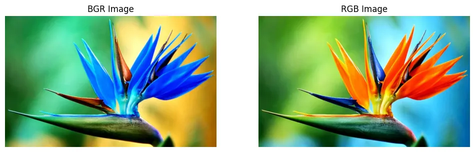
Reading Images

img_flower_bgr = cv.imread('input_files/Strelitzia.jpg')
img_flower_rgb = cv.cvtColor(img_flower_bgr, cv.COLOR_BGR2RGB)

fig, (ax1, ax2) = plt.subplots(1, 2, figsize=(12, 5), sharex=True, sharey=True)

ax1.axis('off')
ax1.imshow(img_flower_bgr)
ax1.set_title('BGR Image')

ax2.axis('off')
ax2.imshow(img_flower_rgb)
ax2.set_title('RGB Image')

plt.savefig('assets/Image_Processing_01.webp', bbox_inches='tight')
plt.show()

Working with Images Cheat Sheet

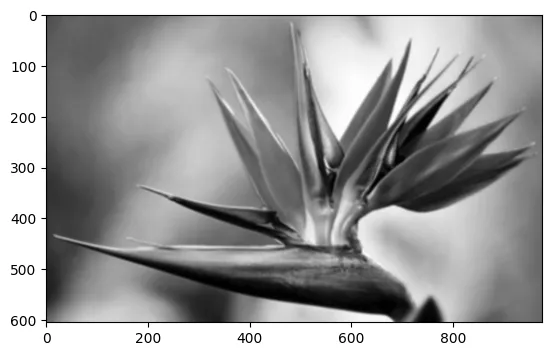
Writing Images

cv.imwrite('input_files/Strelitzia_monochrome.jpg', cv.cvtColor(img_flower_rgb, cv.COLOR_BGR2GRAY))

img_flower_monochrome = cv.imread('input_files/Strelitzia_monochrome.jpg', cv.IMREAD_GRAYSCALE)
plt.imshow(img_flower_monochrome, cmap='gray')
plt.savefig('assets/Image_Processing_02.webp', bbox_inches='tight')

Working with Images Cheat Sheet

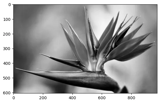
Image Filter

Mean Filter

# image normalized mean filter
filter_norm = np.ones((5,5))/25
filter_norm.shape

img_flower_monochrome.shape

img_flower_monochrome_mean = sciimg.convolve(img_flower_monochrome, filter)
plt.imshow(img_flower_monochrome_mean, cmap='gray')
plt.savefig('assets/Image_Processing_03.webp', bbox_inches='tight')

Working with Images Cheat Sheet

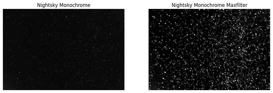
Max Filter

# maximise bright spots
img_stars_monochrome = cv.imread('input_files/nightsky.jpg', cv.IMREAD_GRAYSCALE)
img_stars_monochrome_max = sciimg.maximum_filter(img_stars_monochrome, size=5)

fig, (ax1, ax2) = plt.subplots(1, 2, figsize=(12, 5), sharex=True, sharey=True)

ax1.axis('off')
ax1.imshow(img_stars_monochrome, cmap='gray')
ax1.set_title('Nightsky Monochrome')

ax2.axis('off')
ax2.imshow(img_stars_monochrome_max, cmap='gray')
ax2.set_title('Nightsky Monochrome Maxfilter')

plt.savefig('assets/Image_Processing_04.webp', bbox_inches='tight')

Working with Images Cheat Sheet

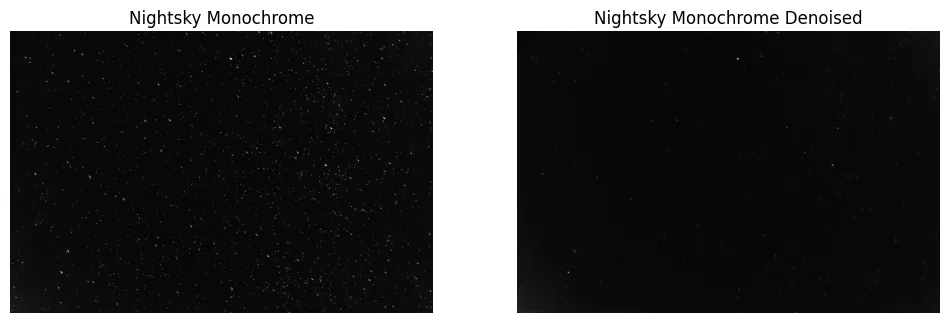
Median Filter

# removing luminance noise
img_stars_denoise = sciimg.median_filter(img_stars_monochrome, size=5)

fig, (ax1, ax2) = plt.subplots(1, 2, figsize=(12, 5), sharex=True, sharey=True)

ax1.axis('off')
ax1.imshow(img_stars_monochrome, cmap='gray')
ax1.set_title('Nightsky Monochrome')

ax2.axis('off')
ax2.imshow(img_stars_denoise, cmap='gray')
ax2.set_title('Nightsky Monochrome Denoised')

plt.savefig('assets/Image_Processing_05.webp', bbox_inches='tight')

Working with Images Cheat Sheet

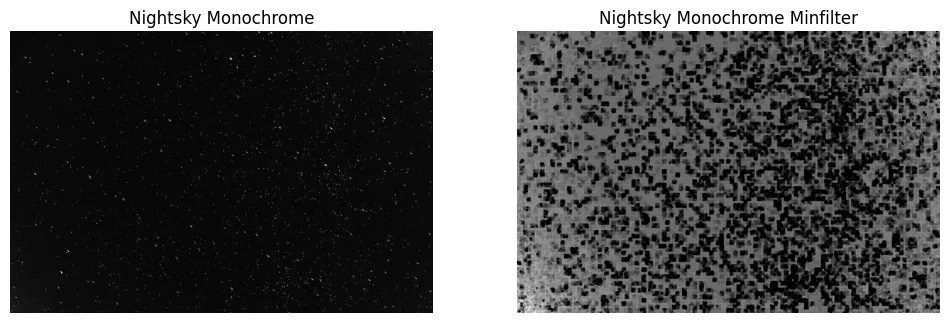
Min Filter

img_stars_monochrome_min = sciimg.minimum_filter(img_stars_monochrome, size=5)

fig, (ax1, ax2) = plt.subplots(1, 2, figsize=(12, 5), sharex=True, sharey=True)

ax1.axis('off')
ax1.imshow(img_stars_monochrome, cmap='gray')
ax1.set_title('Nightsky Monochrome')

ax2.axis('off')
ax2.imshow(img_stars_monochrome_min, cmap='gray')
ax2.set_title('Nightsky Monochrome Minfilter')

plt.savefig('assets/Image_Processing_06.webp', bbox_inches='tight')

Working with Images Cheat Sheet

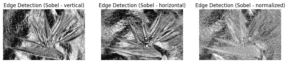
Sobel Filter (Edge Detection)

flower_edge_sobel_h = sciimg.sobel(img_flower_monochrome, 0)
flower_edge_sobel_v = sciimg.sobel(img_flower_monochrome, 1)

magnitude = np.sqrt(flower_edge_sobel_h^2 + flower_edge_sobel_v^2)
magnitude *= 255.0 / np.max(magnitude)  # normalization

fig, (ax1, ax2, ax3) = plt.subplots(1, 3, figsize=(12, 5), sharex=True, sharey=True)

ax1.axis('off')
ax1.imshow(flower_edge_sobel_v, cmap='gray')
ax1.set_title('Edge Detection (Sobel - vertical)')

ax2.axis('off')
ax2.imshow(flower_edge_sobel_h, cmap='gray')
ax2.set_title('Edge Detection (Sobel - horizontal)')

ax3.axis('off')
ax3.imshow(magnitude, cmap='gray')
ax3.set_title('Edge Detection (Sobel - normalized)')

plt.savefig('assets/Image_Processing_07.webp', bbox_inches='tight')

Working with Images Cheat Sheet

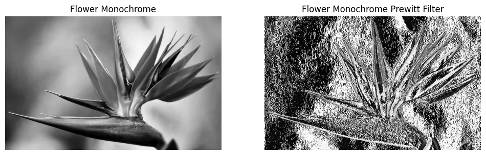
Prewitt Filter (Edge Detection)

flower_edge_prewitt = sciimg.prewitt(img_flower_monochrome)

fig, (ax1, ax2) = plt.subplots(1, 2, figsize=(12, 5), sharex=True, sharey=True)

ax1.axis('off')
ax1.imshow(img_flower_monochrome, cmap='gray')
ax1.set_title('Flower Monochrome')

ax2.axis('off')
ax2.imshow(flower_edge_prewitt, cmap='gray')
ax2.set_title('Flower Monochrome Prewitt Filter')

plt.savefig('assets/Image_Processing_08.webp', bbox_inches='tight')

Working with Images Cheat Sheet

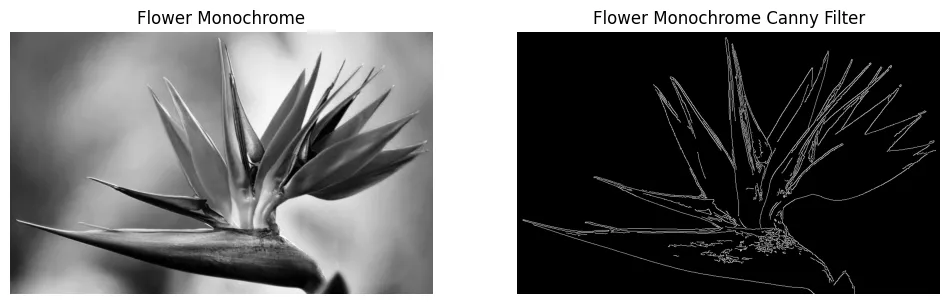
Canny Filter (Edge Detection)

flower_edge_canny = cv.Canny(img_flower_monochrome, 100, 200)

fig, (ax1, ax2) = plt.subplots(1, 2, figsize=(12, 5), sharex=True, sharey=True)

ax1.axis('off')
ax1.imshow(img_flower_monochrome, cmap='gray')
ax1.set_title('Flower Monochrome')

ax2.axis('off')
ax2.imshow(flower_edge_canny, cmap='gray')
ax2.set_title('Flower Monochrome Canny Filter')

plt.savefig('assets/Image_Processing_09.webp', bbox_inches='tight')

Working with Images Cheat Sheet

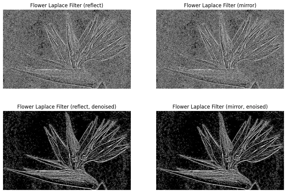
Gaussian Laplace Filter (Edge Detection)

flower_edge_laplace_reflect = sciimg.laplace(img_flower_monochrome, mode='reflect')
flower_edge_laplace_mirror = sciimg.laplace(img_flower_monochrome, mode='mirror')
flower_edge_gaussian_laplace_reflect = sciimg.gaussian_laplace(img_flower_monochrome, sigma=1, mode='reflect')
flower_edge_gaussian_laplace_mirror = sciimg.gaussian_laplace(img_flower_monochrome, sigma=1, mode='mirror')

fig, (ax) = plt.subplots(2, 2, figsize=(12, 8), sharex=True, sharey=True)

ax[0,0].axis('off')
ax[0,0].imshow(flower_edge_laplace_reflect, cmap='gray')
ax[0,0].set_title('Flower Laplace Filter (reflect)')

ax[0,1].axis('off')
ax[0,1].imshow(flower_edge_laplace_mirror, cmap='gray')
ax[0,1].set_title('Flower Laplace Filter (mirror)')

ax[1,0].axis('off')¶
ax[1,0].imshow(flower_edge_gaussian_laplace_reflect, cmap='gray')
ax[1,0].set_title('Flower Laplace Filter (reflect, denoised)')

ax[1,1].axis('off')
ax[1,1].imshow(flower_edge_gaussian_laplace_mirror, cmap='gray')
ax[1,1].set_title('Flower Laplace Filter (mirror, denoised)')

plt.savefig('assets/Image_Processing_10.webp', bbox_inches='tight')

Working with Images Cheat Sheet

Frangi Filter (Shape Detection)

img_klingon_monochrome = cv.imread('input_files/st.jpg', cv.IMREAD_GRAYSCALE)
img_opa_monochrome = cv.imread('input_files/opa.jpg', cv.IMREAD_GRAYSCALE)

klingon_frangi = frangi(
    img_klingon_monochrome,
    black_ridges=False
)
opa_frangi = frangi(
    img_opa_monochrome,
    black_ridges=True
)

fig, (ax1, ax2) = plt.subplots(1, 2, figsize=(12, 5))

ax1.axis('off')
ax1.imshow(klingon_frangi, cmap='gray')
ax1.set_title('Frangi Filter (white ridges)')

ax2.axis('off')
ax2.imshow(opa_frangi, cmap='gray')
ax2.set_title('Frangi Filter (black ridges)')

plt.savefig('assets/Image_Processing_11.webp', bbox_inches='tight')

Working with Images Cheat Sheet

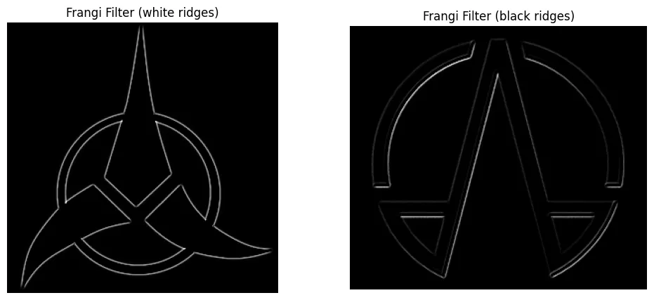
Image Mapping Transformations

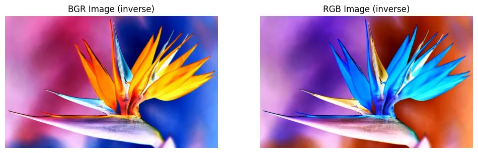
Inverse Transformation

img_flower_rgb_inverse = 255 - img_flower_rgb
img_flower_bgr_inverse = 255 - img_flower_bgr

fig, (ax1, ax2) = plt.subplots(1, 2, figsize=(12, 5), sharex=True, sharey=True)

ax1.axis('off')
ax1.imshow(img_flower_bgr_inverse)
ax1.set_title('BGR Image (inverse)')

ax2.axis('off')
ax2.imshow(img_flower_rgb_inverse)
ax2.set_title('RGB Image (inverse)')

plt.savefig('assets/Image_Processing_12.webp', bbox_inches='tight')

Working with Images Cheat Sheet

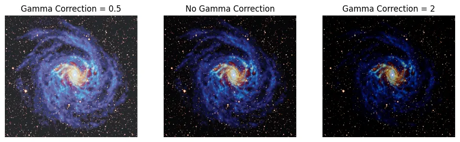
Gamma Correction

gamma1 = 0.5
gamma2 = 2

img_radio_bgr = cv.imread('input_files/deep.png',)
img_radio_rgb = cv.cvtColor(img_radio_bgr, cv.COLOR_BGR2RGB)
img_radio_float = img_radio_rgb.astype(float)

max = np.max(img_radio_float)
img_radio_norm = img_radio_float/max #normalized

gce1 = np.log(img_radio_norm) * gamma1
gamma_correction1 = np.exp(gce1) * 255.0
gamma_int1 = gamma_correction1.astype(int)

gce2 = np.log(img_radio_norm) * gamma2
gamma_correction2 = np.exp(gce2) * 255.0
gamma_int2 = gamma_correction2.astype(int)

fig, ax = plt.subplots(1, 3, figsize=(12, 5), sharex=True, sharey=True)

ax[0].axis('off')
ax[0].imshow(gamma_int1)
ax[0].set_title('Gamma Correction = 0.5')

ax[1].axis('off')
ax[1].imshow(img_radio_rgb)
ax[1].set_title('No Gamma Correction')

ax[2].axis('off')
ax[2].imshow(gamma_int2)
ax[2].set_title('Gamma Correction = 2')

plt.savefig('assets/Image_Processing_13a.webp', bbox_inches='tight')

Working with Images Cheat Sheet

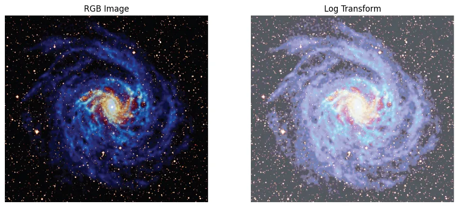
Log Transformation

log_transformation = ( 255.0 * np.log(1 + img_radio_float))/np.log(1 + max)
log_int = log_transformation.astype(int)

fig, (ax1, ax2) = plt.subplots(1, 2, figsize=(12, 5), sharex=True, sharey=True)

ax1.axis('off')
ax1.imshow(img_radio_rgb)
ax1.set_title('RGB Image')

ax2.axis('off')
ax2.imshow(log_int)
ax2.set_title('Log Transform')

plt.savefig('assets/Image_Processing_13b.webp', bbox_inches='tight')

Working with Images Cheat Sheet

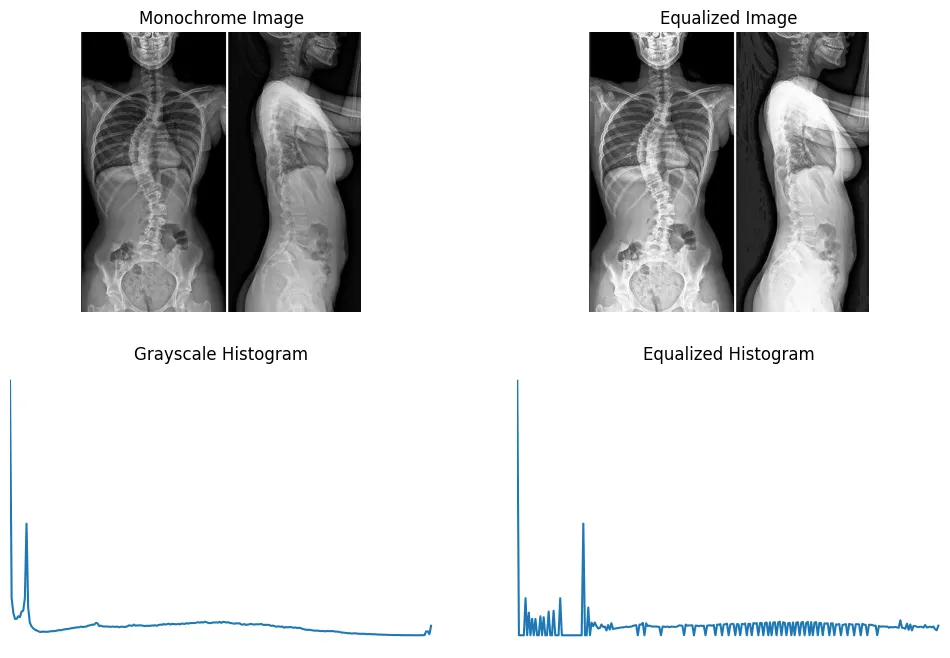
Histogram Equalization

x_ray = cv.imread('input_files/anteroposterior-lateral-views.jpg', cv.IMREAD_GRAYSCALE)
x_ray_equalized = cv.equalizeHist(x_ray)

hist = cv.calcHist([x_ray], [0], None, [256], [0, 256])
hist_eq = cv.calcHist([x_ray_equalized], [0], None, [256], [0, 256])

fig, ax = plt.subplots(2, 2, figsize=(12, 8))

ax[0,0].axis('off')
ax[0,0].imshow(x_ray, cmap='gray')
ax[0,0].set_title('Monochrome Image')

ax[0,1].axis('off')
ax[0,1].imshow(x_ray_equalized, cmap='gray')
ax[0,1].set_title('Equalized Image')

ax[1,0].axis('off')
ax[1,0].set_title("Grayscale Histogram")
ax[1,0].set_xlabel("Bins")
ax[1,0].set_ylabel("# of Pixels")
ax[1,0].plot(hist)
ax[1,0].set_xlim([0, 256])

ax[1,1].axis('off')
ax[1,1].set_title("Equalized Histogram")
ax[1,1].set_xlabel("Bins")
ax[1,1].set_ylabel("# of Pixels")
ax[1,1].plot(hist_eq)
ax[1,1].set_xlim([0, 256])

plt.savefig('assets/Image_Processing_14.webp', bbox_inches='tight')

Working with Images Cheat Sheet

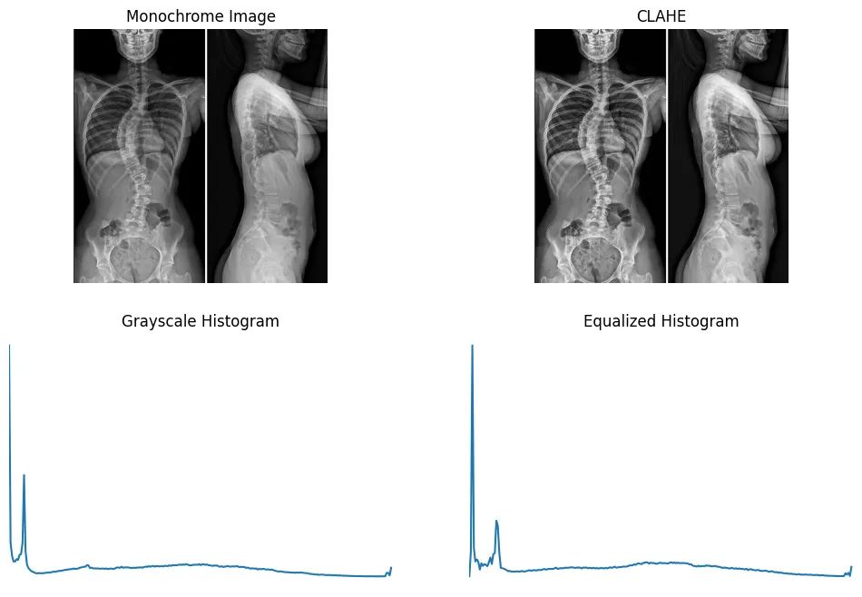
Contrast Limited Adaptive Histogram Equalization (CLAHE)

clahe_eq = cv.createCLAHE(clipLimit=1, tileGridSize=(8,8))
clahe = clahe_eq.apply(x_ray)

hist_eq2 = cv.calcHist([clahe], [0], None, [256], [0, 256])

fig, ax = plt.subplots(2, 2, figsize=(12, 8))

ax[0,0].axis('off')
ax[0,0].imshow(x_ray, cmap='gray')
ax[0,0].set_title('Monochrome Image')

ax[0,1].axis('off')
ax[0,1].imshow(clahe, cmap='gray')
ax[0,1].set_title('CLAHE')

ax[1,0].axis('off')
ax[1,0].set_title("Grayscale Histogram")
ax[1,0].set_xlabel("Bins")
ax[1,0].set_ylabel("# of Pixels")
ax[1,0].plot(hist)
ax[1,0].set_xlim([0, 256])

ax[1,1].axis('off')
ax[1,1].set_title("Equalized Histogram")
ax[1,1].set_xlabel("Bins")
ax[1,1].set_ylabel("# of Pixels")
ax[1,1].plot(hist_eq2)
ax[1,1].set_xlim([0, 256])

plt.savefig('assets/Image_Processing_15.webp', bbox_inches='tight')

Working with Images Cheat Sheet

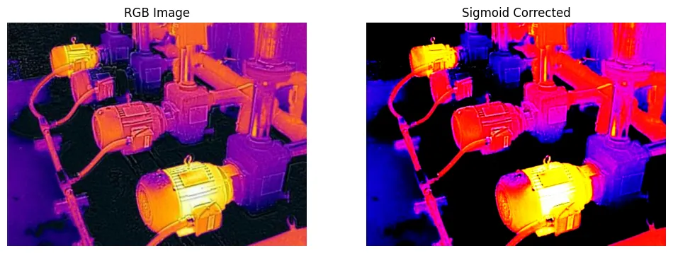
Sigmoid Correction

img_thermal_bgr = cv.imread('input_files/thermal.jpg')
img_thermal_rgb = cv.cvtColor(img_thermal_bgr, cv.COLOR_BGR2RGB)

sigmoid_correction = adjust_sigmoid(img_thermal_rgb, gain=15)

fig, (ax1, ax2) = plt.subplots(1, 2, figsize=(12, 5), sharex=True, sharey=True)

ax1.axis('off')
ax1.imshow(img_thermal_rgb)
ax1.set_title('RGB Image')

ax2.axis('off')
ax2.imshow(sigmoid_correction)
ax2.set_title('Sigmoid Corrected')

plt.savefig('assets/Image_Processing_16.webp', bbox_inches='tight')

Working with Images Cheat Sheet

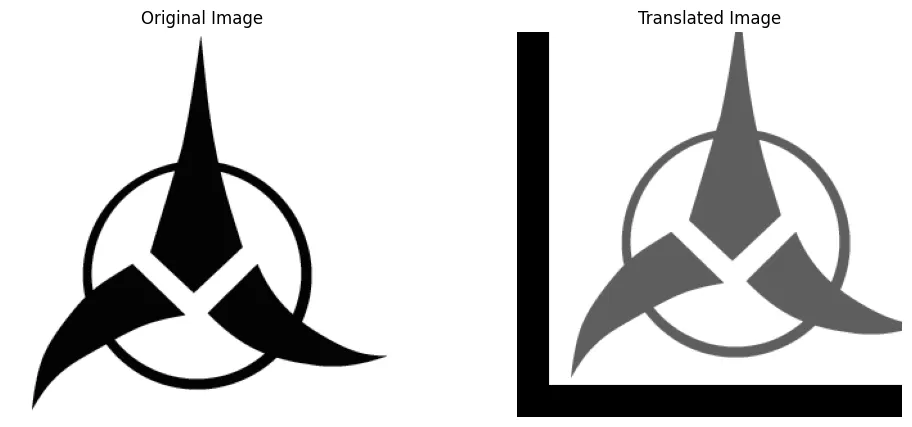
Affine Transformations

Translation

height, width = img_klingon_monochrome.shape[:2]
tx, ty = width/12, height/12

translation_matrix = np.array([
    [1,0,tx],
    [0,1,-ty]
], dtype=np.float32)

translated_image = cv.warpAffine(src=img_klingon_monochrome, M=translation_matrix, dsize=(width,height))

fig, (ax1, ax2) = plt.subplots(1, 2, figsize=(12, 5), sharex=True, sharey=True)

ax1.axis('off')
ax1.imshow(img_klingon_monochrome, cmap='gray')
ax1.set_title('Original Image')

ax2.axis('off')
ax2.imshow(translated_image, cmap='gray')
ax2.set_title('Translated Image')

plt.savefig('assets/Image_Processing_17.webp', bbox_inches='tight')

Working with Images Cheat Sheet

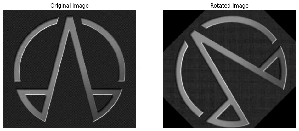
Rotation

height, width = img_opa_monochrome.shape[:2]
center = (width/2, height/2)

rotation_matrix = cv.getRotationMatrix2D(center=center, angle=45, scale=1)

rotated_image = cv.warpAffine(src=img_opa_monochrome, M=rotation_matrix, dsize=(width, height))

fig, (ax1, ax2) = plt.subplots(1, 2, figsize=(12, 5), sharex=True, sharey=True)

ax1.axis('off')
ax1.imshow(img_opa_monochrome, cmap='gray')
ax1.set_title('Original Image')

ax2.axis('off')
ax2.imshow(rotated_image, cmap='gray')
ax2.set_title('Rotated Image')

plt.savefig('assets/Image_Processing_18.webp', bbox_inches='tight')

Working with Images Cheat Sheet

Scaling

shrink_image = cv.resize(img_opa_monochrome, None, fx=0.25, fy=0.25)

squeezed_image = cv.resize(img_opa_monochrome, None, fx=1.5, fy=0.5)

fig, (ax1, ax2) = plt.subplots(1, 2, figsize=(12, 5), sharex=True, sharey=True)

ax1.axis('off')
ax1.imshow(shrink_image, cmap='gray')
ax1.set_title('Shrunken Image')

ax2.axis('off')
ax2.imshow(squeezed_image, cmap='gray')
ax2.set_title('Squeezed Image')

plt.savefig('assets/Image_Processing_19.webp', bbox_inches='tight')

Working with Images Cheat Sheet

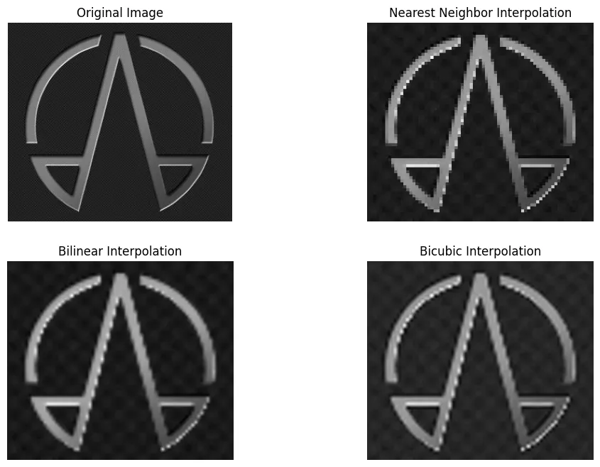
Interpolation

nn_scaling = cv.resize(shrink_image, None, fx=4, fy=4, interpolation=cv.INTER_NEAREST)

bilinear_scaling = cv.resize(shrink_image, None, fx=4, fy=4, interpolation=cv.INTER_LINEAR)

bicubic_scaling = cv.resize(shrink_image, None, fx=4, fy=4, interpolation=cv.INTER_CUBIC)

fig, ax = plt.subplots(2, 2, figsize=(12, 8))

ax[0,0].axis('off')
ax[0,0].imshow(img_opa_monochrome, cmap='gray')
ax[0,0].set_title('Original Image')

ax[0,1].axis('off')
ax[0,1].imshow(nn_scaling, cmap='gray')
ax[0,1].set_title('Nearest Neighbor Interpolation')

ax[1,0].axis('off')
ax[1,0].imshow(bilinear_scaling, cmap='gray')
ax[1,0].set_title('Bilinear Interpolation')

ax[1,1].axis('off')
ax[1,1].imshow(bicubic_scaling, cmap='gray')
ax[1,1].set_title('Bicubic Interpolation')

plt.savefig('assets/Image_Processing_20.webp', bbox_inches='tight')

Working with Images Cheat Sheet

Frequency Filtering

# read in monochrome image
x_img = Image.open('input_files/anteroposterior-lateral-views.jpg').convert('L')

# perform fast fourier transformation
img_fft = fft2(x_img)

# shift fourier frequency image
img_shift = fftshift(img_fft)

w = img_shift.shape[0]
h = img_shift.shape[1]

center1 = w/2
center2 = h/2

cut_off_radius = 30.0

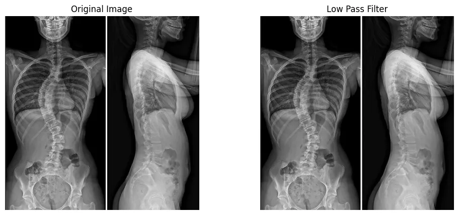
Lowpass Filter

# initialize filter with 1's
filter_lp = np.ones((w,h))

# convolution function
for i in range(1,w):
    for j in range(1,h):
        r1 = (i - center1)**2 + (j - center2)**2
        r = math.sqrt(r1)
        # cut-off high frequencies
        if r > cut_off_radius:
            filter_lp[i,j] == 0.0

# convert filter to image
H_lp = Image.fromarray(filter_lp)

# convolution
conv_lp= img_shift * H_lp

# magnitude of the inverse FFT
mag_inv_lp = abs(ifft2(conv_lp))

fig, (ax1, ax2) = plt.subplots(1, 2, figsize=(12, 5), sharex=True, sharey=True)

ax1.axis('off')
ax1.imshow(x_img, cmap='gray')
ax1.set_title('Original Image')

ax2.axis('off')
ax2.imshow(mag_inv_lp, cmap='gray')
ax2.set_title('Low Pass Filter')

plt.savefig('assets/Image_Processing_21.webp', bbox_inches='tight')

Working with Images Cheat Sheet

Butterworth Lowpass Filter

t1 = 1

# initialize filter with 1's
filter_blp = np.ones((w,h))

# convolution function
for i in range(1,w):
    for j in range(1,h):
        r1 = (i - center1)**2 + (j - center2)**2
        r = math.sqrt(r1)
        # cut-off high frequencies
        if r > cut_off_radius:
            filter_blp[i,j] = 1/(1 + (r/cut_off_radius)**t1)

# convert filter to image
H_blp = Image.fromarray(filter_blp)

# convolution
conv_blp = img_shift * H_blp

# magnitude of the inverse FFT
mag_inv_blp = abs(ifft2(conv_blp))

fig, (ax1, ax2) = plt.subplots(1, 2, figsize=(12, 5), sharex=True, sharey=True)

ax1.axis('off')
ax1.imshow(x_img, cmap='gray')
ax1.set_title('Original Image')

ax2.axis('off')
ax2.imshow(mag_inv_blp, cmap='gray')
ax2.set_title('Butterworth Low Pass Filter')

plt.savefig('assets/Image_Processing_22.webp', bbox_inches='tight')

Working with Images Cheat Sheet

Gaussian Lowpass Filter

t1 = 2*cut_off_radius

# initialize filter with 1's
filter_glp = np.ones((w,h))

# convolution function
for i in range(1,w):
    for j in range(1,h):
        r1 = (i - center1)**2 + (j - center2)**2
        r = math.sqrt(r1)
        # cut-off high frequencies
        if r > cut_off_radius:
            filter_glp[i,j] = math.exp(-r**2/t1**2)

# convert filter to image
H_glp = Image.fromarray(filter_glp)

# convolution
conv_glp = img_shift * H_glp

# magnitude of the inverse FFT
mag_inv_glp = abs(ifft2(conv_glp))

fig, (ax1, ax2) = plt.subplots(1, 2, figsize=(12, 5), sharex=True, sharey=True)

ax1.axis('off')
ax1.imshow(x_img, cmap='gray')
ax1.set_title('Original Image')

ax2.axis('off')
ax2.imshow(mag_inv_glp, cmap='gray')
ax2.set_title('Gaussian Low Pass Filter')

plt.savefig('assets/Image_Processing_23.webp', bbox_inches='tight')

Working with Images Cheat Sheet

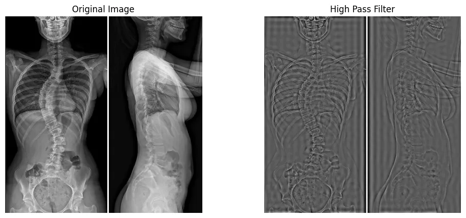
Highpass Filter

filter_hp = np.ones((w,h))

# convolution function
for i in range(1,w):
    for j in range(1,h):
        r1 = (i - center1)**2 + (j - center2)**2
        r = math.sqrt(r1)
        # cut-off low frequencies
        if 0 < r < cut_off_radius:
            filter_hp[i,j] = 0.0

# convert filter to image
H_hp = Image.fromarray(filter_hp)

# convolution
conv_hp = img_shift * H_hp

# magnitude of the inverse FFT
mag_inv_hp = abs(ifft2(conv_hp))

fig, (ax1, ax2) = plt.subplots(1, 2, figsize=(12, 5), sharex=True, sharey=True)

ax1.axis('off')
ax1.imshow(x_img, cmap='gray')
ax1.set_title('Original Image')

ax2.axis('off')
ax2.imshow(mag_inv_hp, cmap='gray')
ax2.set_title('High Pass Filter')

plt.savefig('assets/Image_Processing_24.webp', bbox_inches='tight')

Working with Images Cheat Sheet

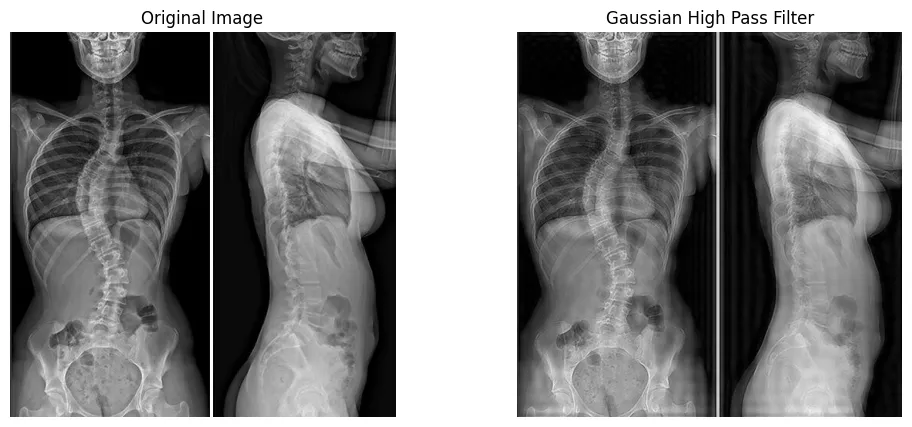
Gaussian Highpass Filter

filter_ghp = np.ones((w,h))

t1 = 2*cut_off_radius

# convolution function
for i in range(1,w):
    for j in range(1,h):
        r1 = (i - center1)**2 + (j - center2)**2
        r = math.sqrt(r1)
        # cut-off high frequencies
        if r > cut_off_radius:
            filter_ghp[i,j] = 1 - math.exp(-r**2/t1**2)

markers=# convert filter to image
H_ghp = Image.fromarray(filter_ghp)

# convolution
conv_ghp = img_shift * H_ghp

# magnitude of the inverse FFT
mag_inv_ghp = abs(ifft2(conv_ghp))

fig, (ax1, ax2) = plt.subplots(1, 2, figsize=(12, 5), sharex=True, sharey=True)

ax1.axis('off')
ax1.imshow(x_img, cmap='gray')
ax1.set_title('Original Image')

ax2.axis('off')
ax2.imshow(mag_inv_ghp, cmap='gray')
ax2.set_title('Gaussian High Pass Filter')

plt.savefig('assets/Image_Processing_25.webp', bbox_inches='tight')

Working with Images Cheat Sheet

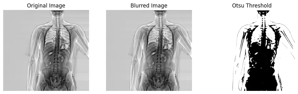
Segmentation

x2_img = cv.imread('input_files/xray.jpg', cv.IMREAD_GRAYSCALE)
x2_img_blur = cv.GaussianBlur(x2_img, (7,7), 0)

Otsu's Method

(T, theshInv) = cv.threshold(x2_img_blur, 0 , 255, cv.THRESH_BINARY | cv.THRESH_OTSU)

fig, (ax1, ax2, ax3) = plt.subplots(1, 3, figsize=(12, 5), sharex=True, sharey=True)

ax1.axis('off')
ax1.imshow(x2_img, cmap='gray')
ax1.set_title('Original Image')

ax2.axis('off')
ax2.imshow(x2_img_blur, cmap='gray')
ax2.set_title('Blurred Image')

ax3.axis('off')
ax3.imshow(theshInv, cmap='gray')
ax3.set_title('Otsu Threshold')

plt.savefig('assets/Image_Processing_26.webp', bbox_inches='tight')

Working with Images Cheat Sheet

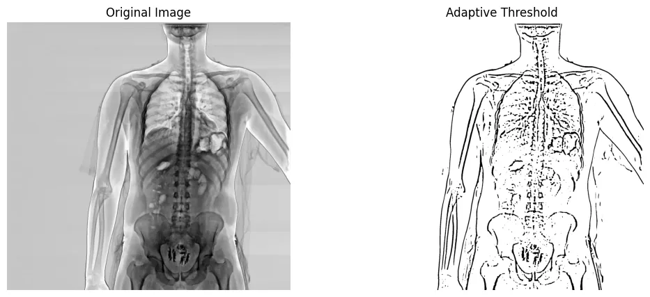
Adaptive Thresholding

adaptive_threshold = cv.adaptiveThreshold(x2_img_blur, 255, cv.ADAPTIVE_THRESH_MEAN_C, cv.THRESH_BINARY, 21, 10)

fig, (ax1, ax2) = plt.subplots(1, 2, figsize=(12, 5), sharex=True, sharey=True)

ax1.axis('off')
ax1.imshow(x2_img, cmap='gray')
ax1.set_title('Original Image')

ax2.axis('off')
ax2.imshow(adaptive_threshold, cmap='gray')
ax2.set_title('Adaptive Threshold')

plt.savefig('assets/Image_Processing_27.webp', bbox_inches='tight')

Working with Images Cheat Sheet

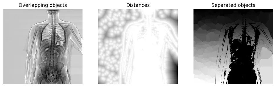
Watershed Segmentation

ret, thresh = cv.threshold(x2_img, 0, 255, cv.THRESH_BINARY + cv.THRESH_OTSU)

distance = sciimg.distance_transform_edt(thresh)
coords = peak_local_max(distance, min_distance=15, footprint=np.ones((3, 3)), labels=thresh)
mask = np.zeros(distance.shape, dtype=bool)
mask[tuple(coords.T)] = True
markers, _ = sciimg.label(mask)

labels = watershed(-distance, markers, mask=thresh)

print("{} unique segments found".format(len(np.unique(labels)) - 1))

fig, axes = plt.subplots(ncols=3, figsize=(12, 5), sharex=True, sharey=True)
ax = axes.ravel()

ax[0].imshow(x2_img, cmap=plt.cm.gray)
ax[0].set_title('Overlapping objects')
ax[1].imshow(-distance, cmap=plt.cm.gray)
ax[1].set_title('Distances')
ax[2].imshow(labels, cmap=plt.cm.gray)
ax[2].set_title('Separated objects')

for a in ax:
    a.set_axis_off()

plt.savefig('assets/Image_Processing_28.webp', bbox_inches='tight')

Working with Images Cheat Sheet

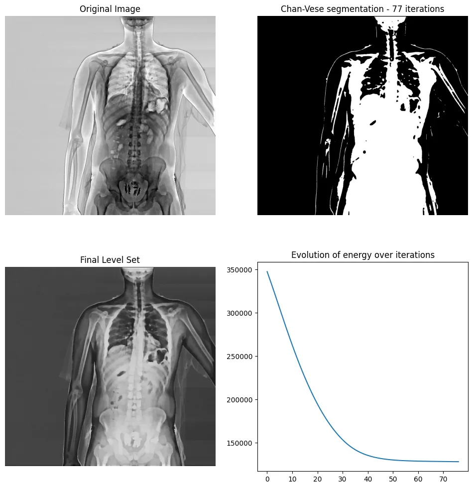
Contour-Based Segmentation

x2_img_float = img_as_float(x2_img)

cv = chan_vese(
    x2_img_float, mu=0.2, lambda1=1, lambda2=1,
    tol=1e-3, max_num_iter=200, dt=0.5,
    init_level_set="checkerboard", extended_output=True
)

fig, axes = plt.subplots(2, 2, figsize=(12, 12))
ax = axes.flatten()

ax[0].imshow(x2_img, cmap="gray")
ax[0].set_axis_off()
ax[0].set_title("Original Image", fontsize=12)

ax[1].imshow(cv[0], cmap="gray")
ax[1].set_axis_off()
title = f'Chan-Vese segmentation - {len(cv[2])} iterations'
ax[1].set_title(title, fontsize=12)

ax[2].imshow(cv[1], cmap="gray")
ax[2].set_axis_off()
ax[2].set_title("Final Level Set", fontsize=12)

ax[3].plot(cv[2])
ax[3].set_title("Evolution of energy over iterations", fontsize=12)

plt.savefig('assets/Image_Processing_29.webp', bbox_inches='tight')

Working with Images Cheat Sheet

Morphing

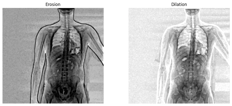
Erosion & Dilation

kernel = np.ones((7,7), np.uint8)

img_eroded = cv.erode(x2_img, kernel, iterations=2)

img_dilated = cv.dilate(x2_img, kernel, iterations=2)

fig, (ax1, ax2) = plt.subplots(1, 2, figsize=(12, 5), sharex=True, sharey=True)

ax1.axis('off')
ax1.imshow(img_eroded, cmap='gray')
ax1.set_title('Erosion')

ax2.axis('off')
ax2.imshow(img_dilated, cmap='gray')
ax2.set_title('Dilation')

plt.savefig('assets/Image_Processing_30.webp', bbox_inches='tight')

Working with Images Cheat Sheet

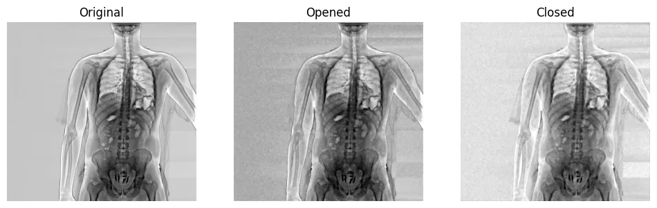
Opening & Closing

Opening: Erosion followed by Dilation
Closing: Dilation followed by Erosion

kernel = cv.getStructuringElement(cv.MORPH_RECT, (9,9))

img_opened = cv.morphologyEx(x2_img, cv.MORPH_OPEN, kernel)

img_closed = cv.morphologyEx(x2_img, cv.MORPH_CLOSE, kernel)

fig, axes = plt.subplots(ncols=3, figsize=(12, 5), sharex=True, sharey=True)
ax = axes.ravel()

ax[0].imshow(x2_img, cmap=plt.cm.gray)
ax[0].set_title('Original')
ax[1].imshow(img_opened, cmap=plt.cm.gray)
ax[1].set_title('Opened')
ax[2].imshow(img_closed, cmap=plt.cm.gray)
ax[2].set_title('Closed')

for a in ax:
    a.set_axis_off()

plt.savefig('assets/Image_Processing_31.webp', bbox_inches='tight')

Working with Images Cheat Sheet

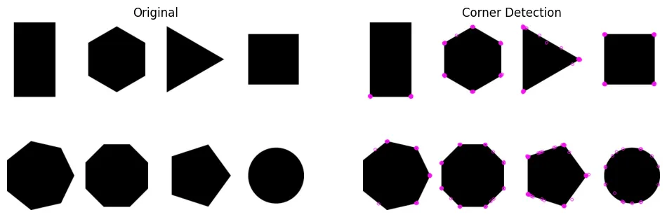
Feature Detection

Fast Corner Detector

img_shapes = cv.imread('input_files/shapes.jpg', cv.IMREAD_GRAYSCALE)

detector = cv.FastFeatureDetector_create()
detector.setNonmaxSuppression(False)

corners = detector.detect(img_shapes, None)
corners_image = cv.drawKeypoints(img_shapes, corners, None, color=(245,20,240))

fig, (ax1, ax2) = plt.subplots(1, 2, figsize=(12, 5), sharex=True, sharey=True)

ax1.axis('off')
ax1.imshow(img_shapes, cmap='gray')
ax1.set_title('Original')

ax2.axis('off')
ax2.imshow(corners_image, cmap='gray')
ax2.set_title('Corner Detection')

plt.savefig('assets/Image_Processing_32.webp', bbox_inches='tight')

Working with Images Cheat Sheet

OpenCV & SciPy and Scikit Image Cheat Sheet

Basic Image Operations​

Reading Images​

Writing Images​

Image Filter​

Mean Filter​

Max Filter​

Median Filter​

Min Filter​

Sobel Filter (Edge Detection)​

Prewitt Filter (Edge Detection)​

Canny Filter (Edge Detection)​

Gaussian Laplace Filter (Edge Detection)​

Frangi Filter (Shape Detection)​

Image Mapping Transformations​

Inverse Transformation​

Gamma Correction​

Log Transformation​

Histogram Equalization​

Contrast Limited Adaptive Histogram Equalization (CLAHE)​

Sigmoid Correction​

Affine Transformations​

Translation​

Rotation​

Scaling​

Interpolation​

Frequency Filtering​

Lowpass Filter​

Butterworth Lowpass Filter​

Gaussian Lowpass Filter​

Highpass Filter​

Gaussian Highpass Filter​

Segmentation​

Otsu's Method​

Adaptive Thresholding​

Watershed Segmentation​

Contour-Based Segmentation​

Morphing​

Erosion & Dilation​

Opening & Closing​

Feature Detection​

Fast Corner Detector​

Basic Image Operations

Reading Images

Writing Images

Image Filter

Mean Filter

Max Filter

Median Filter

Min Filter

Sobel Filter (Edge Detection)

Prewitt Filter (Edge Detection)

Canny Filter (Edge Detection)

Gaussian Laplace Filter (Edge Detection)

Frangi Filter (Shape Detection)

Image Mapping Transformations

Inverse Transformation

Gamma Correction

Log Transformation

Histogram Equalization

Contrast Limited Adaptive Histogram Equalization (CLAHE)

Sigmoid Correction

Affine Transformations

Translation

Rotation

Scaling

Interpolation

Frequency Filtering

Lowpass Filter

Butterworth Lowpass Filter

Gaussian Lowpass Filter

Highpass Filter

Gaussian Highpass Filter

Segmentation

Otsu's Method

Adaptive Thresholding

Watershed Segmentation

Contour-Based Segmentation

Morphing

Erosion & Dilation

Opening & Closing

Feature Detection

Fast Corner Detector