Tensorflow Tensorboard

Tensorboard is - since Tensorflow 2.0 - a build-in model learning dashboard that we can use to track the network performance by accuracy and loss statistics. I want to take my previous project Feature Detection based on the MNIST Fashion Dataset and add Tensorboard to optimize my neural network.
Adding Tensorboard
I will start with the simple network layout that is used by the official Tensorflow tutorial:
classifier = tf.keras.Sequential([
  tf.keras.layers.Conv2D(input_shape=(28,28,1), filters=8, kernel_size=3, strides=2, activation='relu', name='Conv1'),
  tf.keras.layers.Flatten(),
  tf.keras.layers.Dense(10, name='Dense')
])

classifier.compile(optimizer='adam',
  loss=tf.keras.losses.SparseCategoricalCrossentropy(from_logits=True),
  metrics=[tf.keras.metrics.SparseCategoricalAccuracy()])
Now before starting the training we have to add two lines to initialize Tensorboard and insert this callback into our training:
# configuring tensorboard
log_dir="tensorboard/logs/" + datetime.datetime.now().strftime("%Y%m%d-%H%M%S")
tensorboard_callback = tf.keras.callbacks.TensorBoard(log_dir=log_dir, histogram_freq=1)

# model training
classifier.fit(X_train, y_train, epochs=EPOCHS, callbacks=[tensorboard_callback])
Starting Tensorboard
To execute Tensorboard run the following command in your terminal or add the following line to the end of your training code:
# execute tensorboard
os.system("tensorboard --logdir tensorboard/logs")
This will serve Tensorboard on port 6006:
Serving TensorBoard on localhost; to expose to the network, use a proxy or pass --bind_all
TensorBoard 2.11.0 at http://localhost:6006/ (Press CTRL+C to quit)
A brief overview of the dashboards shown (tabs in top navigation bar):
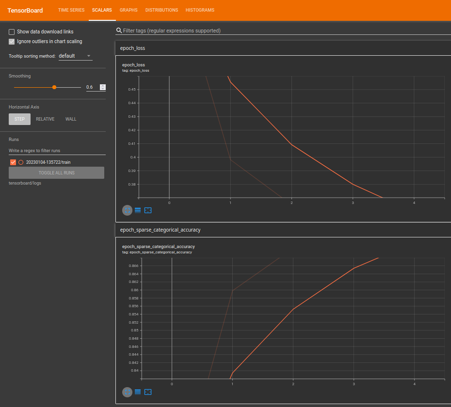
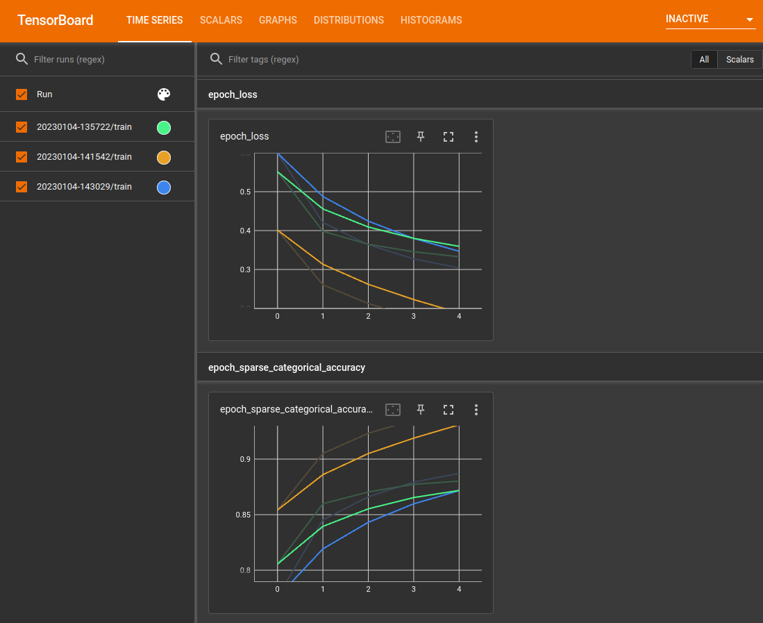
- The Scalars dashboard shows how the loss and metrics change with every epoch. You can use it to also track training speed, learning rate, and other scalar values.
- The Graphs dashboard helps you visualize your model. In this case, the Keras graph of layers is shown which can help you ensure it is built correctly.
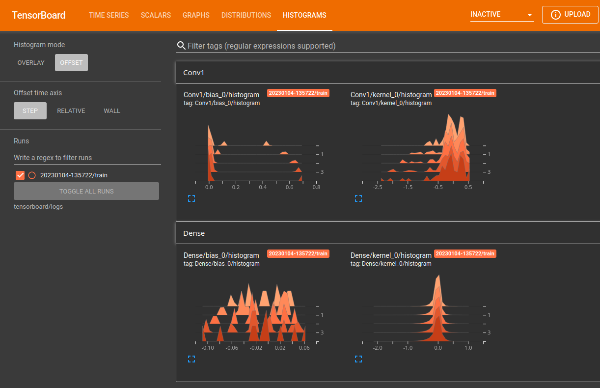
- The Distributions and Histograms dashboards show the distribution of a Tensor over time. This can be useful to visualize weights and biases and verify that they are changing in an expected way.
Tracking Progress
Changing to a slightly more complicated network:
## second attempt
classifier = tf.keras.Sequential([
  tf.keras.layers.Conv2D(32, (3,3), activation = 'relu', input_shape = (28,28,1)),
  tf.keras.layers.MaxPooling2D(2,2),
  tf.keras.layers.Conv2D(64, (3, 3), activation='relu'),
  tf.keras.layers.Flatten(),
  tf.keras.layers.Dense(64, activation = 'relu'),
  tf.keras.layers.Dense(10, activation = 'softmax')
])
The first attempt in green and the second in orange it is already very obvious that the latter performs a lot better:
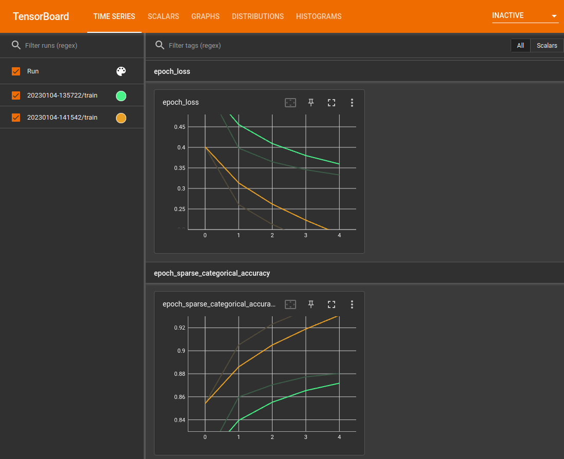
So add even more complexity and see what happens:
## third attempt
classifier = tf.keras.Sequential([
  tf.keras.layers.Conv2D(6, (5,5), activation = 'relu', input_shape = (28,28,1)),
  tf.keras.layers.AveragePooling2D(),
  tf.keras.layers.Conv2D(16, (5,5), activation = 'relu'),
  tf.keras.layers.AveragePooling2D(),
  tf.keras.layers.Flatten(),
  tf.keras.layers.Dense(120, activation = 'relu'),
  tf.keras.layers.Dense(84, activation = 'relu'),
  tf.keras.layers.Dense(10, activation = 'softmax')
])
We can see that this network (blue) roughly performs as well as the first attempt network (green) - in this case I would continue working with the second network (orange) as it performs significantly better:
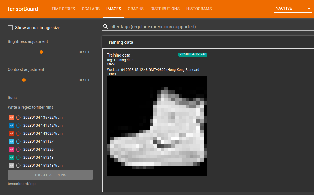
Displaying Image Datasets
To be able to inspect images from our dataset in Tensorboard we need to add an file_writer. The following will take the first image of the training dataset and make it available to Tensorboard:
# configuring tensorboard
## set log data location
log_dir="tensorboard/logs/" + datetime.datetime.now().strftime("%Y%m%d-%H%M%S")
## create a file writer for the log directory
file_writer = tf.summary.create_file_writer(log_dir)
## reshape the first training image
img = np.reshape(X_train[0], (-1, 28, 28, 1))
## using the file writer to log the reshaped image
with file_writer.as_default():
  tf.summary.image("Training data", img, step=0)
## create Tensorboard callback
tensorboard_callback = tf.keras.callbacks.TensorBoard(log_dir=log_dir, histogram_freq=1)
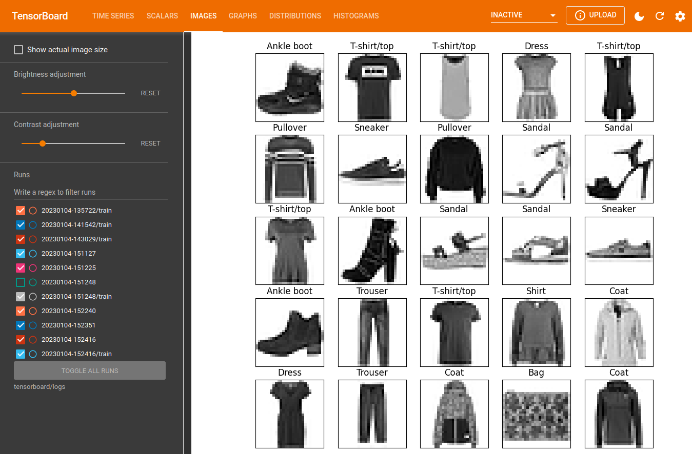
Logging arbitrary Image Data
In the code below, you'll log the first 25 images as a nice grid using matplotlib's subplot() function:
# configuring tensorboard
## set log data location
log_dir="tensorboard/logs/" + datetime.datetime.now().strftime("%Y%m%d-%H%M%S")
## create a file writer for the log directory
file_writer = tf.summary.create_file_writer(log_dir)

def plot_to_image(figure):
  # Converts the matplotlib plot specified by 'figure' to a PNG image and
  # returns it. The supplied figure is closed and inaccessible after this call.
  # Save the plot to a PNG in memory.
  buf = io.BytesIO()
  plt.savefig(buf, format='png')
  # Closing the figure prevents it from being displayed directly inside
  # the notebook.
  plt.close(figure)
  buf.seek(0)
  # Convert PNG buffer to TF image
  image = tf.image.decode_png(buf.getvalue(), channels=4)
  # Add the batch dimension
  image = tf.expand_dims(image, 0)
  return image

def image_grid():
  # Return a 5x5 grid of the MNIST images as a matplotlib figure.
  # Create a figure to contain the plot.
  figure = plt.figure(figsize=(10,10))
  for i in range(25):
    # Start next subplot.
    plt.subplot(5, 5, i + 1, title=class_names[y_train[i]])
    plt.xticks([])
    plt.yticks([])
    plt.grid(False)
    plt.imshow(X_train[i], cmap=plt.cm.binary)

  return figure

# Prepare the plot
figure = image_grid()
# Convert to image and log
with file_writer.as_default():
  tf.summary.image("Training data", plot_to_image(figure), step=0)
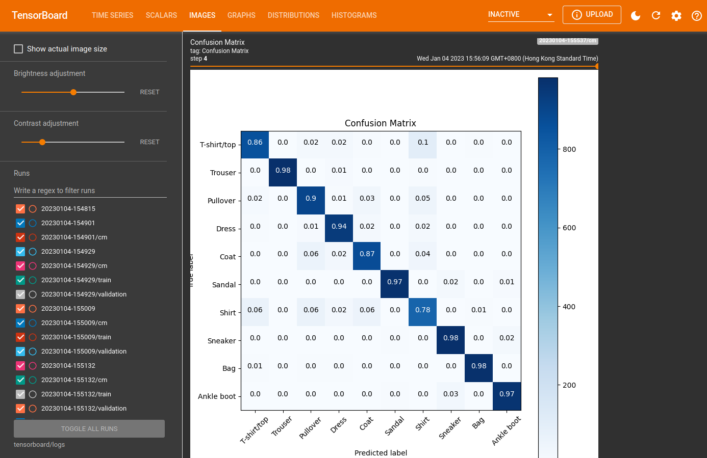
Confusion Matrix
When training a classifier, it's useful to see the confusion matrix. The confusion matrix gives you detailed knowledge of how your classifier is performing on test data. Define a function that calculates the confusion matrix:
def plot_confusion_matrix(cm, class_names):
  """
  Returns a matplotlib figure containing the plotted confusion matrix.

  Args:
    cm (array, shape = [n, n]): a confusion matrix of integer classes
    class_names (array, shape = [n]): String names of the integer classes
  """
  figure = plt.figure(figsize=(8, 8))
  plt.imshow(cm, interpolation='nearest', cmap=plt.cm.Blues)
  plt.title("Confusion Matrix")
  plt.colorbar()
  tick_marks = np.arange(len(class_names))
  plt.xticks(tick_marks, class_names, rotation=45)
  plt.yticks(tick_marks, class_names)

  # Compute the labels from the normalized confusion matrix.
  labels = np.around(cm.astype('float') / cm.sum(axis=1)[:, np.newaxis], decimals=2)

  # Use white text if squares are dark; otherwise black.
  threshold = cm.max() / 2.
  for i, j in itertools.product(range(cm.shape[0]), range(cm.shape[1])):
    color = "white" if cm[i, j] > threshold else "black"
    plt.text(j, i, labels[i, j], horizontalalignment="center", color=color)

  plt.tight_layout()
  plt.ylabel('True label')
  plt.xlabel('Predicted label')
  return figure

file_writer_cm = tf.summary.create_file_writer(log_dir + '/cm')


def log_confusion_matrix(epoch, logs):
  # Use the model to predict the values from the validation dataset.
  test_pred_raw = classifier.predict(X_test)
  test_pred = np.argmax(test_pred_raw, axis=1)

  # Calculate the confusion matrix.
  cm = confusion_matrix(y_test, test_pred)
  # Log the confusion matrix as an image summary.
  figure = plot_confusion_matrix(cm, class_names=class_names)
  cm_image = plot_to_image(figure)

  # Log the confusion matrix as an image summary.
  with file_writer_cm.as_default():
    tf.summary.image("Confusion Matrix", cm_image, step=epoch)

# Define the per-epoch callback.
cm_callback = tf.keras.callbacks.LambdaCallback(on_epoch_end=log_confusion_matrix)