AutoML with AutoGluon for Timeseries Forecasts

• Part 1: AutoML with AutoGluon for Tabular Data
• Part 2: AutoML with AutoGluon for Multi-Modal Data
• Part 3: AutoML with AutoGluon for Timeseries Forecasts

AutoGluon automates machine learning tasks enabling you to easily achieve strong predictive performance in your applications. With just a few lines of code, you can train and deploy high-accuracy machine learning and deep learning models on image, text, time series, and tabular data.

Github Repository

• AutoML with AutoGluon for Timeseries Forecasts
  • Installation
  • Single Variate Forecasting
    • Data Preprocessing
    • Model Training
    • Model Evaluation
      • Visualization
  • Multi Variate Forecasting - Future Covariants
    • Data Preprocessing
    • Model Training
    • Model Predictions
      • Visualization
  • Multi Variate Forecasting - Past Covariants
    • Data Preprocessing
    • Model Training
    • Model Predictions
      • Visualization

Installation

Installing AutoGluon with GPU support:

pip install -U pip
pip install -U setuptools wheel
pip install torch==1.13.1+cu117 torchvision==0.14.1+cu117 --extra-index-url https://download.pytorch.org/whl/cu117
pip install autogluon
# for visualizations
pip install bokeh==2.0.1"

Single Variate Forecasting

# get dataset
!wget https://raw.githubusercontent.com/databricks/Spark-The-Definitive-Guide/master/data/retail-data/all/online-retail-dataset.csv -P dataset

from autogluon.timeseries import TimeSeriesDataFrame, TimeSeriesPredictor
import matplotlib.pyplot as plt
from datetime import datetime as dt
import pandas as pd
import seaborn as sns

SEED = 42
MODEL_PATH = 'model'

Data Preprocessing

df = pd.read_csv('dataset/online-retail-dataset.csv')
df.head(5)

	InvoiceNo	StockCode	Description	Quantity	InvoiceDate	UnitPrice	CustomerID	Country
0	536365	85123A	WHITE HANGING HEART T-LIGHT HOLDER	6	12/1/2010 8:26	2.55	17850.0	United Kingdom
1	536365	71053	WHITE METAL LANTERN	6	12/1/2010 8:26	3.39	17850.0	United Kingdom
2	536365	84406B	CREAM CUPID HEARTS COAT HANGER	8	12/1/2010 8:26	2.75	17850.0	United Kingdom
3	536365	84029G	KNITTED UNION FLAG HOT WATER BOTTLE	6	12/1/2010 8:26	3.39	17850.0	United Kingdom
4	536365	84029E	RED WOOLLY HOTTIE WHITE HEART.	6	12/1/2010 8:26	3.39	17850.0	United Kingdom

df.info()
# <class 'pandas.core.frame.DataFrame'>
# RangeIndex: 541909 entries, 0 to 541908
# Data columns (total 8 columns):
#  #   Column       Non-Null Count   Dtype  
# ---  ------       --------------   -----  
#  0   InvoiceNo    541909 non-null  object 
#  1   StockCode    541909 non-null  object 
#  2   Description  540455 non-null  object 
#  3   Quantity     541909 non-null  int64  
#  4   InvoiceDate  541909 non-null  object 
#  5   UnitPrice    541909 non-null  float64
#  6   CustomerID   406829 non-null  float64
#  7   Country      541909 non-null  object 
# dtypes: float64(2), int64(1), object(5)
# memory usage: 33.1+ MB

# only sample last 10.000 items
# df_sample = df.iloc[-10000:]
# take all items
df_sample = df.copy()

# renaming columns
df_sample.rename(columns={'InvoiceNo': 'item_id', 'InvoiceDate': 'timestamp'}, inplace=True)
# create sale total price
df_sample['target'] = df_sample['Quantity'] * df_sample['UnitPrice']
df_sample['item_id'] = 'online_sales'
# create single variant timeseries
df_sample.drop(
    ['StockCode', 'Description', 'CustomerID', 'Country', 'Quantity', 'UnitPrice'],
    axis=1, inplace=True)
df_sample.head(5)

	item_id	timestamp	target
0	online_sales	12/1/2010 8:26	20.40
1	online_sales	12/1/2010 8:26	27.80
2	online_sales	12/1/2010 8:26	2.60
3	online_sales	12/1/2010 8:26	5.85
4	online_sales	12/1/2010 8:26	19.90

# reformat timestamp to remove time from date
df_sample['timestamp'] = pd.to_datetime(df_sample['timestamp']).dt.strftime('%m/%d/%Y')
df_sample.head(5)

	item_id	target	timestamp
0	online_sales	16.6	12/23/2010
1	online_sales	8.5	12/23/2010
2	online_sales	20.8	12/23/2010
3	online_sales	20.8	12/23/2010
4	online_sales	20.8	12/23/2010

# groupby date and sum() up the sales
df_sample = df_sample.groupby(
    ['item_id', 'timestamp']).sum()

print(df_sample.info())
# MultiIndex: 305 entries, ('online_sales', '01/04/2011') to ('online_sales', '12/23/2010')
df_sample.head(5)

item_id	timestamp	target
online_sales	01/04/2011	15584.29
	01/05/2011	75076.22
	01/07/2011	81417.78
	01/09/2011	32131.53

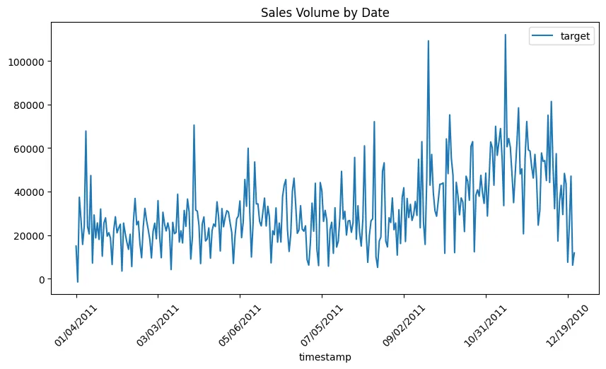
df_sample.loc['online_sales']['target'].plot(
    title='Sales Volume by Date',
    figsize=(10,5),
    rot=45,
    legend=True
)
plt.savefig('assets/AutoGluon_AutoML_TimeSeries_01.webp', bbox_inches='tight')

df_sample.to_csv('dataset/single_variant_ts.csv', index=True)

Model Training

ValueError: Frequency not provided and cannot be inferred. This is often due to the time index of the data being irregularly sampled. Please ensure that the data set used has a uniform time index, or create the TimeSeriesPredictor setting ignore_time_index=True.

AutoGluon does not like irregular timeseries AT ALL... I manually fixed the timestamp column with regular, daily interval. Docs recommend auto-filling for missing data before model training.

train_data = TimeSeriesDataFrame('dataset/single_variant_ts.csv')
train_data.describe()

	target
count	305.000000
mean	31959.829292
std	17414.261664
min	-1566.230000
25%	20728.140000
50%	27978.410000
75%	42912.400000
max	112141.110000

# create a predictor for 30 days (30 row in dataset) forcast
sv_predictor = TimeSeriesPredictor(
    prediction_length=30,
    path=MODEL_PATH,
    target='target',
    eval_metric='sMAPE'
)

sv_predictor.fit(
    train_data,
    time_limit=800,
    presets="medium_quality"
)

# Training complete. Models trained: ['Naive', 'SeasonalNaive', 'Theta', 'AutoETS', 'RecursiveTabular', 'DeepAR', 'WeightedEnsemble']
# Total runtime: 146.36 s
# Best model: WeightedEnsemble
# Best model score: -0.2301

sv_predictor.fit_summary()

Estimated performance of each model:

	model	score_val	pred_time_val	fit_time_marginal	fit_order
0	WeightedEnsemble	-0.321595	1.042651	1.881647	7
1	RecursiveTabular	-0.321595	1.042651	0.757291	5
2	DeepAR	-0.384756	0.095033	69.751811	6
3	AutoETS	-0.385364	22.865800	0.012004	4
4	Theta	-0.397785	24.269135	0.009619	3
5	SeasonalNaive	-0.403544	5.162711	0.010179	2
6	Naive	-0.403544	5.572433	0.009085	1
Number of models trained: 7
Types of models trained:
{'MultiWindowBacktestingModel', 'TimeSeriesGreedyEnsemble'}

Model Evaluation

# return a 1 month forcast on the training data
sv_predictions = sv_predictor.predict(train_data, random_seed=SEED)

sv_predictions

		mean	0.1	0.2	0.3	0.4	0.5	0.6	0.7	0.8	0.9
item_id	timestamp
online_sales	2011-10-16	35231.549892	14821.287291	21889.080854	26885.810628	31139.108555	35389.176845	39525.311786	43747.076754	48715.574839	55619.827997
	2011-10-17	37319.098400	9315.489680	18992.518673	25927.428089	31800.990269	37256.964611	42685.962390	48685.278476	55741.918605	65278.986905
	2011-10-18	38623.633612	5142.371285	16610.764052	24909.974641	32018.253338	38569.692694	45201.922577	52390.855571	60646.930906	72387.928409
	2011-10-19	40741.301758	1946.154973	15539.068760	25137.953113	33223.044572	40765.606934	48463.165389	56628.990736	66077.743741	79722.836483
	2011-10-20	49296.101707	6303.232915	21458.815514	31910.941266	40964.792632	49394.712059	57908.461563	66841.601504	77474.686240	92186.915812
	2011-10-21	42399.179004	-4222.418692	11966.114749	23324.147218	33287.622759	42457.754199	51587.049946	61400.403661	72842.296970	88931.093472
	2011-10-22	33619.926637	-17087.154419	364.144617	12901.404480	23491.862364	33662.238893	43520.884464	54164.964907	66630.573647	84037.471194
	2011-10-23	39042.384772	-14703.540432	3853.552955	17218.430626	28519.710014	39090.598639	49763.392538	60939.668264	74324.111121	92676.374673
	2011-10-24	37314.733017	-19270.824930	233.744114	14092.680263	26011.109933	37258.663681	48286.522116	60254.494754	74152.628169	93725.394967
	2011-10-25	40035.277581	-19730.031575	823.364529	15754.378083	28379.185360	40095.125237	51768.504080	64369.746415	78969.545369	99392.125068
	2011-10-26	43809.551647	-18581.300915	2831.155428	18233.929143	31493.221895	43799.325572	56059.960500	69262.074053	84846.687611	106247.592685
	2011-10-27	40978.233969	-24604.018712	-2246.682396	14204.335705	28124.915072	41120.107016	53865.685435	67632.214997	83850.112737	106498.851884
	2011-10-28	41743.192227	-26024.978536	-2645.385307	14166.811130	28273.284258	41561.178311	54943.112404	69180.700278	86004.451402	109515.329421
	2011-10-29	38315.939169	-32037.733749	-7961.047361	9530.292590	24433.420394	38430.213583	52199.831968	67014.321833	84580.597330	108781.710477
	2011-10-30	40790.730787	-31714.294692	-6632.032918	11250.135692	26624.395493	40830.333814	55083.397136	70254.854690	88116.212266	113018.777994
	2011-10-31	39601.428364	-35269.325656	-9299.692907	9073.426874	24982.993094	39702.658833	54402.247423	70171.210127	88614.257154	114229.722423
	2011-11-01	43321.091336	-33495.290752	-7238.416761	11718.451027	27982.345746	43267.875515	58529.011730	74809.030961	93805.173651	120492.849400
	2011-11-02	39873.310897	-39638.237188	-12259.488831	7259.635658	24107.774345	39944.400252	55573.550817	72172.974172	91871.915068	119270.200045
	2011-11-03	38897.212691	-42509.220460	-14725.370733	5465.492686	22784.085743	38756.254195	54814.426553	72198.679766	92621.915745	120534.229094
	2011-11-04	45310.748490	-37919.694783	-9357.164960	11175.946162	28815.300995	45152.634721	61626.068300	79239.016639	99980.063552	128811.104239
	2011-11-05	40524.113111	-45095.463685	-15760.925828	5668.926472	23679.488279	40503.121411	57398.500638	75497.467474	96633.997752	126117.225307
	2011-11-06	40806.692620	-46676.736613	-16544.120931	5068.030397	23563.217104	40845.487542	58063.833664	76565.798203	98222.894111	128465.220975
	2011-11-07	43503.676450	-46255.703438	-15315.077993	6965.648074	25902.252457	43336.311215	61053.512552	80111.716545	102295.131332	133194.560977
	2011-11-08	39830.233893	-51545.615185	-20027.924158	2662.824619	21906.346012	39980.482428	58006.295602	77399.156839	99888.163672	131151.589197
	2011-11-09	36990.513044	-56523.526649	-24495.447993	-1066.945972	18732.001915	37151.279157	55520.419680	75331.859267	98382.970785	130468.262942
	2011-11-10	42656.625332	-52222.084277	-19714.514788	3802.223665	23887.046793	42525.441250	61225.057142	81332.468161	104820.044505	137808.305522
	2011-11-11	44756.329828	-52548.031615	-18656.197064	5288.754038	25734.360637	44828.240961	63986.351020	84378.816506	108611.618683	142140.108263
	2011-11-12	37905.655743	-60991.102805	-27099.347751	-2388.499412	18511.776221	38050.389629	57546.974229	78416.261580	102719.966853	136415.925032
	2011-11-13	44715.800505	-55633.323514	-20782.285358	3913.667987	24980.451031	44809.798552	64605.937576	85704.112222	110433.920792	144866.205041
	2011-11-14	38863.458282	-62877.590928	-28234.112477	-2844.261356	18802.531926	38951.660430	59170.908563	80678.533877	105966.185779	141098.465744

Visualization

def plot_predictions(train_data, predictions, item_id, target_column, titel, ylabel):
    plt.figure(figsize=(12,5))
    plt.title(titel)
    plt.xlabel('Date')
    plt.ylabel(ylabel)
    # timeseries data
    y_train = train_data.loc[item_id][target_column]
    plt.plot(y_train, label="Timeseries Data")
    # forcast data
    y_pred = predictions.loc[item_id]
    plt.plot(y_pred['mean'], label="Mean Forecast")
    # confidence intervals
    plt.fill_between(
        y_pred.index , y_pred['0.1'], y_pred['0.9'],
        color='red', alpha=0.1, label='10%-90% Confidence Range'
    )

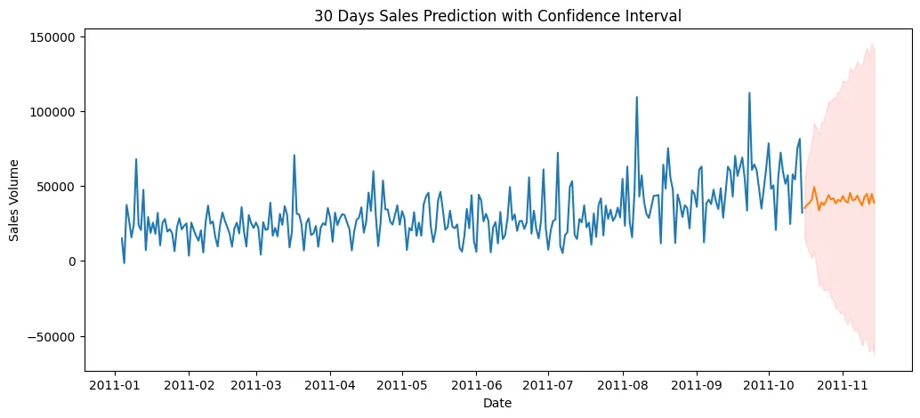
plot_predictions(
    train_data, sv_predictions,
    item_id='online_sales', target_column='target',
    titel='30 Days Sales Prediction with Confidence Interval',
    ylabel = 'Sales Volume'
)
plt.savefig('assets/AutoGluon_AutoML_TimeSeries_02.webp', bbox_inches='tight')

Multi Variate Forecasting - Future Covariants

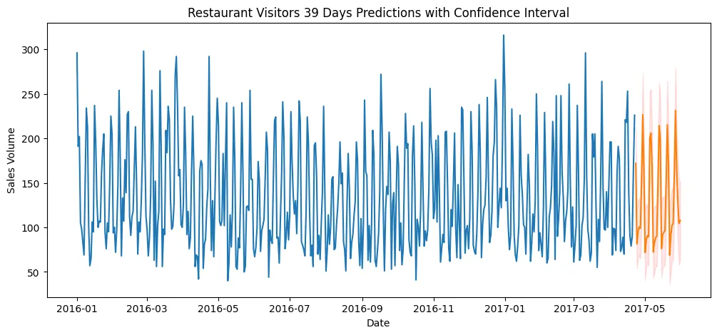
Add known factors that affected your time series data in the past to future prediction - e.g. holidays on restaurant revenues.

# get dataset
!wget https://github.com/DaviRolim/datasets/raw/master/RestaurantVisitors.csv -P dataset

Data Preprocessing

df = pd.read_csv('dataset/RestaurantVisitors.csv')
df.tail(5)
# dataset contains unknowns -> will be used for prediction

	date	weekday	holiday	holiday_name	rest1	rest2	rest3	rest4	total
512	5/27/2017	Saturday	0	na	NaN	NaN	NaN	NaN	NaN
513	5/28/2017	Sunday	0	na	NaN	NaN	NaN	NaN	NaN
514	5/29/2017	Monday	1	Memorial Day	NaN	NaN	NaN	NaN	NaN
515	5/30/2017	Tuesday	0	na	NaN	NaN	NaN	NaN	NaN
516	5/31/2017	Wednesday	0	na	NaN	NaN	NaN	NaN	NaN

df.info()
# there are `517` entries but only `478` have a total

	Column	Non-Null Count	Dtype
0	date		517 non-null
1	weekday	517 non-null	object
2	holiday	517 non-null	int64
3	holiday_name	517 non-null	object
4	rest1	478 non-null	float64
5	rest2	478 non-null	float64
6	rest3	478 non-null	float64
7	rest4	478 non-null	float64
8	total	478 non-null	float64

df_sample = df.copy()

# renaming columns
df_sample.rename(columns={'total': 'target', 'date': 'timestamp'}, inplace=True)
df_sample['item_id'] = 'restaurant_visitors'

# get numeric representation of weekday from timestamp
datetimes = pd.to_datetime(df_sample['timestamp'])
df_sample['timestamp'] = datetimes
df_sample['weekday'] = datetimes.dt.day_of_week

# drop not needed
df_sample.drop(
    ['rest1', 'rest2', 'rest3', 'rest4', 'holiday_name'],
    axis=1, inplace=True)

df_sample.tail(5)

	timestamp	weekday	holiday	target	item_id
512	2017-05-27	5	0	NaN	restaurant_visitors
513	2017-05-28	6	0	NaN	restaurant_visitors
514	2017-05-29	0	1	NaN	restaurant_visitors
515	2017-05-30	1	0	NaN	restaurant_visitors
516	2017-05-31	2	0	NaN	restaurant_visitors

# split missing data for prediction
df_sample.iloc[:478].to_csv('dataset/mv_known_series.csv', index=False)
df_sample.iloc[478:].drop('target',axis=1).to_csv('dataset/mv_unknown_series.csv', index=False)

Model Training

train_data = TimeSeriesDataFrame('dataset/mv_known_series.csv')
train_data.head(5)

		weekday	holiday	target
item_id	timestamp
restaurant_visitors	2016-01-01	4	1	296.0
	2016-01-02	5	0	191.0
	2016-01-03	6	0	202.0
	2016-01-04	0	0	105.0
	2016-01-05	1	0	98.0

# create a predictor for the length of the unknown series
mv_predictor = TimeSeriesPredictor(
    prediction_length=len(df_sample.iloc[478:]),
    path=MODEL_PATH,
    target='target',
    known_covariates_names = ['weekday', 'holiday'],
    eval_metric='sMAPE'
)

mv_predictor.fit(
    train_data,
    time_limit=800,
    presets="high_quality"
)

# Training complete. Models trained: ['Naive', 'SeasonalNaive', 'Theta', 'AutoETS', 'RecursiveTabular', 'DeepAR', 'TemporalFusionTransformer', 'PatchTST', 'AutoARIMA', 'WeightedEnsemble']
# Total runtime: 470.02 s
# Best model: WeightedEnsemble
# Best model score: -0.1501

Model Predictions

future_series = TimeSeriesDataFrame('dataset/mv_unknown_series.csv')

future_series.head(5)

		weekday	holiday
item_id	timestamp
restaurant_visitors	2017-04-23	6	0
	2017-04-24	0	0
	2017-04-25	1	0
	2017-04-26	2	0
	2017-04-27	3	0

mv_predictions = mv_predictor.predict(train_data, known_covariates=future_series, random_seed=SEED)

Visualization

plot_predictions(
    train_data, mv_predictions,
    item_id='restaurant_visitors', target_column='target',
    titel='Restaurant Visitors 39 Days Predictions with Confidence Interval',
    ylabel = 'Restaurant Revenue'
)
plt.savefig('assets/AutoGluon_AutoML_TimeSeries_03.webp', bbox_inches='tight')

Multi Variate Forecasting - Past Covariants

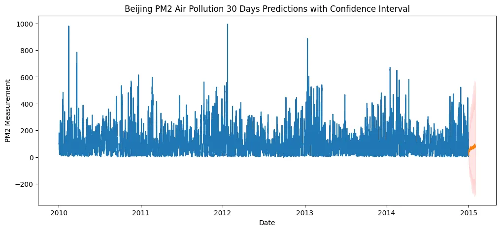
The Air Quality dataset reports on the weather and the level of pollution each hour for five years at the US embassy in Beijing, China. The data includes the date-time, the PM2.5 concentration, and the weather information including dew point, temperature, pressure, wind direction, wind speed and the cumulative number of hours of snow and rain.

# get dataset
!wget https://raw.githubusercontent.com/jyoti0225/Air-Pollution-Forecasting/master/AirPollution.csv -P dataset

Data Preprocessing

# datetime is split up into 4 columns => combine
def parse(x):
    return dt.strptime(x, '%Y %m %d %H')

df = pd.read_csv('dataset/AirPollution.csv', date_parser=parse,parse_dates=[
    ['year', 'month', 'day', 'hour']
])

df.head(5)

	year_month_day_hour	No	pm2.5	DEWP	TEMP	PRES	cbwd	Iws	Is	Ir
0	2010-01-01 00:00:00	1	NaN	-21	-11.0	1021.0	NW	1.79	0	0
1	2010-01-01 01:00:00	2	NaN	-21	-12.0	1020.0	NW	4.92	0	0
2	2010-01-01 02:00:00	3	NaN	-21	-11.0	1019.0	NW	6.71	0	0
3	2010-01-01 03:00:00	4	NaN	-21	-14.0	1019.0	NW	9.84	0	0
4	2010-01-01 04:00:00	5	NaN	-20	-12.0	1018.0	NW	12.97	0	0

df.info()
# dataset contains missing pm2.5 values

#  #   Column               Non-Null Count  Dtype         
# ---  ------               --------------  -----         
#  0   year_month_day_hour  43824 non-null  datetime64[ns]
#  1   No                   43824 non-null  int64         
#  2   pm2.5                41757 non-null  float64       
#  3   DEWP                 43824 non-null  int64         
#  4   TEMP                 43824 non-null  float64       
#  5   PRES                 43824 non-null  float64       
#  6   cbwd                 43824 non-null  object        
#  7   Iws                  43824 non-null  float64       
#  8   Is                   43824 non-null  int64         
#  9   Ir                   43824 non-null  int64 

df_sample = df.copy()

# one-hot encode wind direction
one_hot_wind = pd.get_dummies(df['cbwd'], drop_first=True)
df_sample = pd.concat([df, one_hot_wind], axis=1, join="inner")

# renaming columns
df_sample.rename(columns={
    'year_month_day_hour': 'timestamp',
    'pm2.5': 'target',
    'DEWP': 'dew_point',
    'TEMP': 'temperature',
    'PRES': 'pressure',
    'NW': 'wind_direction_nw',
    'SE': 'wind_direction_se',
    'cv': 'wind_direction_cv',
    'Iws': 'wind_speed',
    'Is': 'snow',
    'Ir': 'rain'}, inplace=True)

# add item_id
df_sample['item_id'] = 'pm2_pollution'

# fill missing targets with mean()
df_sample['target'] = df_sample['target'].fillna(df_sample['target'].mean())

# make datetime object
datetimes = pd.to_datetime(df_sample['timestamp'])
df_sample['timestamp'] = datetimes
df_sample['weekday'] = datetimes.dt.day_of_week

# drop not needed
df_sample.drop(['No', 'cbwd'], axis=1, inplace=True)

df_sample.head(5)

	timestamp	target	dew_point	temperature	pressure	wind_speed	snow	rain	wind_direction_nw	wind_direction_se	wind_direction_cv	item_id	weekday
0	2010-01-01 00:00:00	98.613215	-21	-11.0	1021.0	1.79	0	0	1	0	0	pm2_pollution	4
1	2010-01-01 01:00:00	98.613215	-21	-12.0	1020.0	4.92	0	0	1	0	0	pm2_pollution	4
2	2010-01-01 02:00:00	98.613215	-21	-11.0	1019.0	6.71	0	0	1	0	0	pm2_pollution	4
3	2010-01-01 03:00:00	98.613215	-21	-14.0	1019.0	9.84	0	0	1	0	0	pm2_pollution	4
4	2010-01-01 04:00:00	98.613215	-20	-12.0	1018.0	12.97	0	0	1	0	0	pm2_pollution	4

df_sample.to_csv('dataset/bj_airpollution.csv', index=False)

Model Training

train_data = TimeSeriesDataFrame('dataset/bj_airpollution.csv')
train_data.head(5)

		target	dew_point	temperature	pressure	wind_speed	snow	rain	wind_direction_nw	wind_direction_se	wind_direction_cv	weekday
item_id	timestamp
pm2_pollution	2010-01-01 00:00:00	98.613215	-21	-11.0	1021.0	1.79	0	0	1	0	0	4
	2010-01-01 01:00:00	98.613215	-21	-12.0	1020.0	4.92	0	0	1	0	0	4
	2010-01-01 02:00:00	98.613215	-21	-11.0	1019.0	6.71	0	0	1	0	0	4
	2010-01-01 03:00:00	98.613215	-21	-14.0	1019.0	9.84	0	0	1	0	0	4
	2010-01-01 04:00:00	98.613215	-20	-12.0	1018.0	12.97	0	0	1	0	0	4

# 30-day predictor
bj_predictor = TimeSeriesPredictor(
    prediction_length=24*30,
    path=MODEL_PATH,
    target='target',
    eval_metric='sMAPE'
)

bj_predictor.fit(
    train_data,
    presets="high_quality"
)

# Fitting simple weighted ensemble.
# 	-0.8465       = Validation score (-sMAPE)
# 	3.16    s     = Training runtime
# 	40.20   s     = Validation (prediction) runtime
# Training complete. Models trained: ['Naive', 'SeasonalNaive', 'Theta', 'AutoETS', 'RecursiveTabular', 'DeepAR', 'PatchTST', 'AutoARIMA', 'WeightedEnsemble']
# Total runtime: 693.53 s
# Best model: WeightedEnsemble
# Best model score: -0.8465

Model Predictions

bj_predictions = bj_predictor.predict(train_data, random_seed=SEED)

Visualization

plot_predictions(
    train_data, bj_predictions,
    item_id='pm2_pollution', target_column='target',
    titel='Beijing PM2 Air Pollution 30 Days Predictions with Confidence Interval',
    ylabel = 'PM2 Measurement'
)
plt.savefig('assets/AutoGluon_AutoML_TimeSeries_04.webp', bbox_inches='tight')