Deep Audio

- Signal Processing with Tensorflow
- Project Setup
- Data Loading
- Creating the Dataset
- Calculating Average Length of a Birdcall
- Converting Data into a Spectrogram
- Preparing a Testing & Training Dataset
- Build the Deep Learning Model
- Training the Model
- Making Predictions
- Putting the Model to Work
- Processing the RAW Data
Signal Processing with Tensorflow
The Challenge is to build a Machine Learning model and code to count the number of Capuchinbird calls within a given clip. This can be done in a variety of ways and we would recommend that you do some research into various methods of audio recognition.
Project Setup
The Dataset is provided on kaggle.com and contains of three sets of bird call recordings:
- raw (RAW Data)
- positives (Cut out positive bird calls)
- negatives (Cut out negatives)
Copy them into your data folder. Open a Jupyter Notebook and create a notebook called signal-processing:
jupyter notebook
Now we can install the Python dependencies from inside the notebook:
!pip install tensorflow tensorflow-gpu tensorflow-io matplotlib
Once installed import them into your notebook:
import os
from matplotlib import pyplot as plt
import tensorflow as tf
import tensorflow_io as tfio
Data Loading
To work with the recorded audio files we can select the corresponding data paths - in the example below we pick both an example file that contains the signal we are looking for and one that only comes with background noise:
CAPUCHIN_FILE = os.path.join('data', 'positives', 'XC3776-3.wav')
NOT_CAPUCHIN_FILE = os.path.join('data', 'negatives', 'afternoon-birds-song-in-forest-0.wav')
And read a single audio stream (mono) resampled to 16kHz from those files by feeding the filepath into the following function:
- decode_wav : Read single channel from stereo file
- squeeze : Since all the data is single channel (mono), drop the
channelsaxis from array - resample : Reduce audio data to 16kHz
def load_wav_16k_mono(filename):
    # Load encoded wav file
    file_contents = tf.io.read_file(filename)
    # Decode wav (tensors by channels)
    wav, sample_rate = tf.audio.decode_wav(file_contents, desired_channels=1)
    # Removes trailing axis
    wav = tf.squeeze(wav, axis=-1)
    sample_rate = tf.cast(sample_rate, dtype=tf.int64)
    # Goes from 44100Hz to 16000hz - amplitude of the audio signal
    wav = tfio.audio.resample(wav, rate_in=sample_rate, rate_out=16000)
    return wav
We can run the function over both the positive and negative file:
wave = load_wav_16k_mono(CAPUCHIN_FILE)
nwave = load_wav_16k_mono(NOT_CAPUCHIN_FILE)
And overlay both waves in a plot:
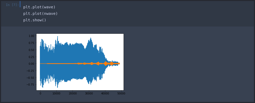
The blue plot represents the positive signal - the correct bird call. While the orange plot is a negative representing our baseline background noise. This now gives us a image representation of our audio that we can use to train our neural network with.
Creating the Dataset
First we need to define the path to all our positive and negative audio files:
POS = os.path.join('data', 'positives')
NEG = os.path.join('data', 'negatives')
Now we can store all the data paths inside Tensorflow Datasets:
pos = tf.data.Dataset.list_files(POS+'/*.wav')
neg = tf.data.Dataset.list_files(NEG+'/*.wav')
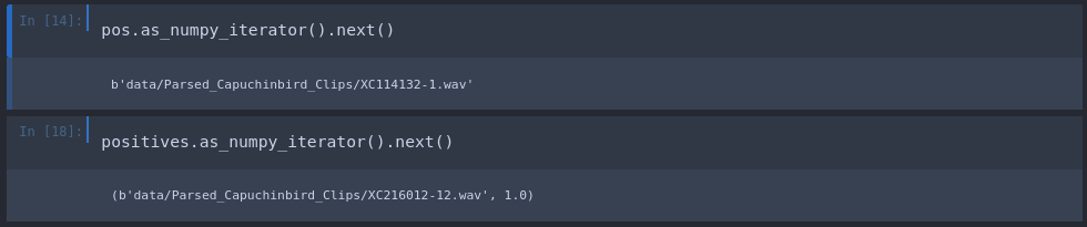
We can now label our data by adding ones and zeros to each filepath inside the dataset depending on whether it is a positive or negative sample:
positives = tf.data.Dataset.zip((pos, tf.data.Dataset.from_tensor_slices(tf.ones(len(pos)))))

negatives = tf.data.Dataset.zip((neg, tf.data.Dataset.from_tensor_slices(tf.zeros(len(neg)))))
After successfully labelling our data we can now merge everything into a single dataset:
data = positives.concatenate(negatives)
Calculating Average Length of a Birdcall
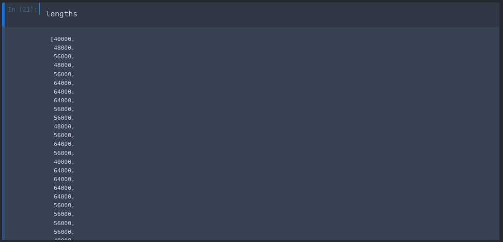
To be able to count bird calls in our RAW data we first have to know the average length of a single call. We can do this by taking all our parsed positive recordings and load them into their waveform:
lengths = []
for file in os.listdir(os.path.join('data', 'positives')):
    tensor_wave = load_wav_16k_mono(os.path.join('data', 'positives', file))
    lengths.append(len(tensor_wave))
By appending each file length to the lengths array we can now do some basic maths to calculate the Min, Max and AVG length of a positive birdcall:
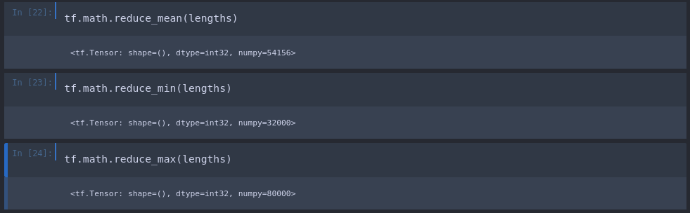
This means that the average birdcall ist 54156 / 16000 Hz = 3.38s. And the calls are in between Min 2s and Max 5s in length.
Converting Data into a Spectrogram
The following function takes an audio file and converts it to 16 kHz Mono. Since we know that the average call is about 3s in length we can limit our data to the first 48000 units of each parsed audio file.
Since our minimum file length was 32000 we need to make sure that every file is padded up with zeros to a length of 48000 using the tf.zeros function:
def preprocess(file_path, label):
	# Load files into 16kHz mono
    wav = load_wav_16k_mono(file_path)
    # Only read the first 3 secs
    wav = wav[:48000]
    # If file < 3s add zeros
    zero_padding = tf.zeros([48000] - tf.shape(wav), dtype=tf.float32)
    wav = tf.concat([zero_padding, wav],0)
    # Use Short-time Fourier Transform
    spectrogram = tf.signal.stft(wav, frame_length=320, frame_step=32)
    # Convert to absolut values (no negatives)
    spectrogram = tf.abs(spectrogram)
    # Add channel dimension (needed by CNN later)
    spectrogram = tf.expand_dims(spectrogram, axis=2)
    return spectrogram, label
To create the spectrogram we can use the Short-time Fourier Transformation provided by Tensorflow.
_Note: the dimensions of each spectrogram are 1491,257,1 - which represents the height and width of the image representation + an additional channel that was added with the tf.expand_dims function. This channel does not hold any information here but is expected to exists by the Tensorflow model we are going to use later.
Test Function
Pick a random audio file from the positives dataset:
filepath, label = positives.shuffle(buffer_size=10000).as_numpy_iterator().next()
And run it through the pre-processing function:
spectrogram, label = preprocess(filepath, label)
Let's see what the spectrum actually looks like:
plt.figure(figsize=(30,20))
plt.imshow(tf.transpose(spectrogram)[0])
plt.show()
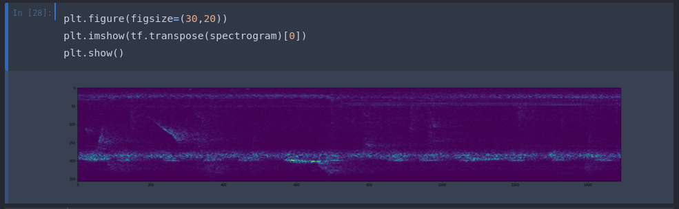
For comparison, this is the spectrogram of a negative sample:
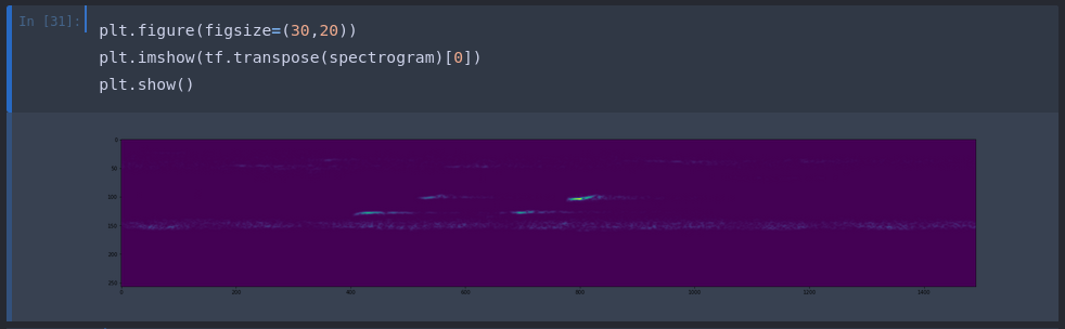
Now all we have to do, is to train a Tensorflow model that is able to distinguish between those two image representation of our audio data.
Preparing a Testing & Training Dataset
We already wrapped all of our data - positives and negatives - into the data variable. So now we can map through this data and feed each file to the preprocessing function.
data = data.map(preprocess)
data = data.cache()
data = data.shuffle(buffer_size=1000)
data = data.batch(16)
data = data.prefetch(8)
To optimize the training we will first shuffle the data and limit the amount of simultaneous files being processed to 16 and the pre-fetch to 8 files. This can be increased if your CPU/GPU can handle it.
To split our data into training and testing data we can run:
train = data.take(36)
test = data.skip(36).take(15)
With len(data) = 51 the split ration is close to 70:30. We can verify the content of each array by:
Training Set
samples, labels = train.as_numpy_iterator().next
labels

array([0., 0., 1., 0., 0., 0., 1., 0., 0., 0., 0., 0., 0., 0., 0., 1.],
      dtype=float32)
Testing Set
samples, labels = test.as_numpy_iterator().next()
labels

array([0., 0., 1., 0., 0., 1., 1., 0., 0., 0., 1., 0., 1., 0., 1., 0.],
      dtype=float32)
Build the Deep Learning Model
from tensorflow.keras.models import Sequential
from tensorflow.keras.layers import Conv2D, Dense, Flatten
Sequential Model
model = Sequential()
model.add(Conv2D(8, (3,3), activation='relu', input_shape=(1491,257,1)))
model.add(Conv2D(8, (3,3), activation='relu'))
model.add(Flatten())
model.add(Dense(32, activation='relu'))
model.add(Dense(1, activation='sigmoid'))
model.compile('Adam', loss='BinaryCrossentropy', metrics=[tf.keras.metrics.Recall(),tf.keras.metrics.Precision()])
model.summary()
Model: "sequential"
_________________________________________________________________
 Layer (type)                Output Shape              Param #
=================================================================
 conv2d (Conv2D)             (None, 1489, 255, 8)      80

 conv2d_1 (Conv2D)           (None, 1487, 253, 8)      584

 flatten (Flatten)           (None, 3009688)           0

 dense (Dense)               (None, 32)                96310048

 dense_1 (Dense)             (None, 1)                 33

=================================================================
Total params: 96,310,745
Trainable params: 96,310,745
Non-trainable params: 0
_________________________________________________________________
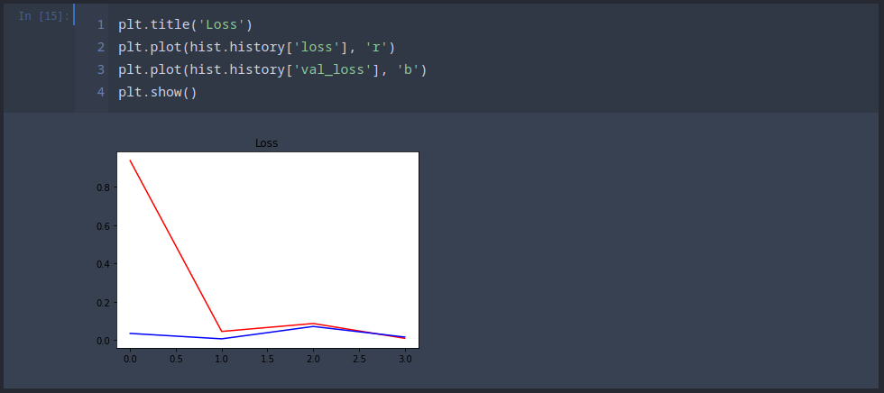
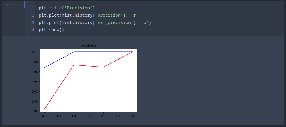
Training the Model
hist = model.fit(train, epochs=4, validation_data=test)
Already after 4 epochs we are starting to get getting a precision and recall value around 100%:
Epoch 4/4
36/36 [==============================] - 6s 177ms/step - loss: 0.0091 - recall: 0.9870 - precision: 1.0000 - val_loss: 0.0157 - val_recall: 0.9844 - val_precision: 1.0000
Making Predictions
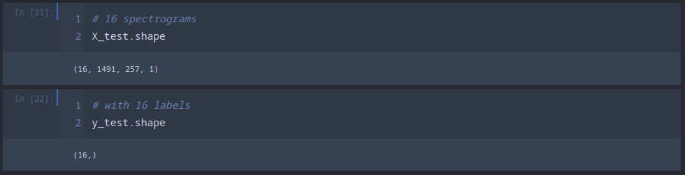
We can now use our testing data - the 16 files we excluded from the training dataset - and use them to run a prediction against:
X_test, y_test = test.as_numpy_iterator().next()
The yhat parameter gives us the probabilities of a file being the recording of a birdcall:
yhat = model.predict(X_test)
Every value that is close to 1.00000000e+00 is a recording that, with a very high probability, contains the birdcall we are looking for:
array([[9.99920249e-01],
       [3.07901189e-08],
       [1.00000000e+00],
       [2.84484369e-25],
       [9.62874225e-09],
       [9.99707282e-01],
       [1.53503152e-05],
       [2.34340667e-03],
       [8.77155067e-28],
       [1.00000000e+00],
       [1.14530545e-08],
       [5.61734714e-06],
       [3.27430301e-20],
       [1.99461836e-11],
       [0.00000000e+00],
       [0.00000000e+00]], dtype=float32)
To make this more readable we can make this - within a selected range of confidence - binary:
yhat = [1 if prediction > 0.5 else 0 for prediction in yhat]
Which looks like this:
[1, 0, 1, 0, 0, 1, 0, 0, 0, 1, 0, 0, 0, 0, 0, 0]
We can verify that this result is correct by calculating the sum of yhat and comparing it with the sum of y_test - which are our labels that we set to 1 for positives and 0 for negatives:
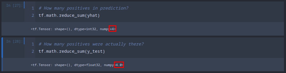
And it seems that we were able to identify all 4 of them! But we should also rule out false-positives/negatives by comparing both arrays:
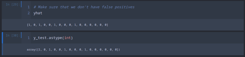
And we have a match - all the zeros and ones are where they belong.
Putting the Model to Work
We now have a well performing model that is able to recognize bird calls. So we can now let it loose on the RAW forest recordings in the data/raw directory. First we need a function that loads the recordings - that are this time in mp3 containers. So instead of the tf.io.read_file function we now need to use tfio.audio.AudioIOTensor. We will handle the stereo recording by adding both channels into a single channel and divide every value by 2:
def load_mp3_16k_mono(filename):
    # Load a WAV file, convert it to a float tensor, resample to 16 kHz single-channel audio.
    res = tfio.audio.AudioIOTensor(filename)
    # Convert to tensor and combine channels
    tensor = res.to_tensor()
    tensor = tf.math.reduce_sum(tensor, axis=1) / 2
    # Extract sample rate and cast
    sample_rate = res.rate
    sample_rate = tf.cast(sample_rate, dtype=tf.int64)
    # Resample to 16 kHz
    wav = tfio.audio.resample(tensor, rate_in=sample_rate, rate_out=16000)
    return wav
Test Function
We can test the loading function by loading a single file:
mp3 = os.path.join('data', 'Forest Recordings', 'recording_00.mp3')
wav = load_mp3_16k_mono(mp3)
Since the RAW recordings are much longer than the neatly parsed training recordings that were already cut down to the length of a typical bird call we can now slice up the file into short sequences of the same length 48000:
audio_slices = tf.keras.utils.timeseries_dataset_from_array(wav, wav, sequence_length=48000, sequence_stride=48000, batch_size=1)
We can check the amount of slices that were generated with len(audio_slices) - and in case of the file recording_00.mp3 we end up with 60 sequences.
Data Preprocessing
The pre-processing step is identical to before. We can pick the first sequence out of the 60 slices that were generated, make sure that it is the correct length (which of course in case of the first slice - it will be). And then continue generating the spectrogram:
def preprocess_mp3(sample, index):
    sample = sample[0]
    zero_padding = tf.zeros([48000] - tf.shape(sample), dtype=tf.float32)
    wav = tf.concat([zero_padding, sample],0)
    spectrogram = tf.signal.stft(wav, frame_length=320, frame_step=32)
    spectrogram = tf.abs(spectrogram)
    spectrogram = tf.expand_dims(spectrogram, axis=2)
    return spectrogram
Now we can create the audio slices and run them through the preprocessing function:
audio_slices = tf.keras.utils.timeseries_dataset_from_array(wav, wav, sequence_length=48000, sequence_stride=48000, batch_size=1)
audio_slices = audio_slices.map(preprocess_mp3)
audio_slices = audio_slices.batch(64)
Running a Prediction
With the 60 slices in place we can now run our prediction model against them - this time I will bump up the confidence to 90% to make sure we don't catch any background noise:
yhat = model.predict(audio_slices)
yhat = [1 if prediction > 0.9 else 0 for prediction in yhat]
The yhat variable now returns 60 zeros and ones depending on wether the tested sequence contained a bird call or not:
len(yhat)
60

yhat
[0,0,0,1,1,0,0,0,0,0,0,0,0,1,1,0,0,0,0,0,0,0,0,1,1,0,0,0,0,0,0,0,0,0,0,0,1,0,0,0,0,0,0,0,0,1,1,0,0,0,0,0,0,0,0,0,0,0,0,0]
But we can see that there are consecutive detections that are most likely caused by us slicing a single bird call into two. Currently we would count't 8 bird calls:
tf.math.reduce_sum(yhat)
<tf.Tensor: shape=(), dtype=int32, numpy=8>
Grouping Consecutive Hits
from itertools import groupby

yhat = [key for key, group in groupby(yhat)]
calls = tf.math.reduce_sum(yhat).numpy()
This reduces the number of detections to 5 - which we can confirm by listening to the recording_00.mp3 file and counting using finger technology:
calls
5
Processing the RAW Data
Now with everything in place we can loop through every file in the raw directory and count our detections:
results = {}
for file in os.listdir(os.path.join('data', 'raw')):
    FILEPATH = os.path.join('data','raw', file)

    wav = load_mp3_16k_mono(FILEPATH)
    audio_slices = tf.keras.utils.timeseries_dataset_from_array(wav, wav, sequence_length=48000, sequence_stride=48000, batch_size=1)
    audio_slices = audio_slices.map(preprocess_mp3)
    audio_slices = audio_slices.batch(64)

    yhat = model.predict(audio_slices)

    results[file] = yhat
This returns predictions for every slice in every recording:
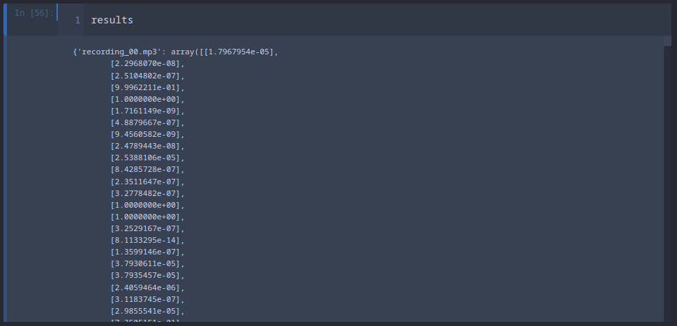
Again we can make this more readable by turning everything with a 99% confidence into ones and the rest into zeros:
class_preds = {}
for file, logits in results.items():
    class_preds[file] = [1 if prediction > 0.99 else 0 for prediction in logits]
class_preds
And group all consecutive detections to make sure we don't double-count them:
postprocessed = {}
for file, scores in class_preds.items():
    postprocessed[file] = tf.math.reduce_sum([key for key, group in groupby(scores)]).numpy()
postprocessed
Now we end up with the sum of all calls inside each file:
{'recording_00.mp3': 5,
 'recording_01.mp3': 0,
 'recording_02.mp3': 0,
 'recording_03.mp3': 0,
 'recording_04.mp3': 4,
 'recording_05.mp3': 0,
 'recording_06.mp3': 5,
 'recording_07.mp3': 2,
 'recording_08.mp3': 25,
 'recording_09.mp3': 0,
 'recording_10.mp3': 5,
 'recording_11.mp3': 3,
 'recording_12.mp3': 0,
 'recording_13.mp3': 0,
 'recording_14.mp3': 0,
 'recording_15.mp3': 2,
 'recording_17.mp3': 3,
 'recording_18.mp3': 5,
 'recording_19.mp3': 0,
 'recording_20.mp3': 0,
 'recording_21.mp3': 1,
 'recording_22.mp3': 2,
 'recording_23.mp3': 5,
 'recording_24.mp3': 0,
 'recording_25.mp3': 16,
 'recording_26.mp3': 2,
 'recording_27.mp3': 0,
 'recording_28.mp3': 16,
 'recording_29.mp3': 0,
 'recording_30.mp3': 2,
 'recording_31.mp3': 1,
 'recording_32.mp3': 2,
 'recording_34.mp3': 4,
 'recording_35.mp3': 0,
 'recording_36.mp3': 0,
 'recording_37.mp3': 3,
 'recording_38.mp3': 1,
 'recording_39.mp3': 9,
 'recording_40.mp3': 1,
 'recording_41.mp3': 0,
 'recording_42.mp3': 0,
 'recording_43.mp3': 5,
 'recording_44.mp3': 1,
 'recording_45.mp3': 3,
 'recording_46.mp3': 17,
 'recording_47.mp3': 16,
 'recording_48.mp3': 4,
 'recording_49.mp3': 0,
 'recording_51.mp3': 3,
 'recording_52.mp3': 0,
 'recording_53.mp3': 0,
 'recording_54.mp3': 3,
 'recording_55.mp3': 0,
 'recording_56.mp3': 16,
 'recording_57.mp3': 3,
 'recording_58.mp3': 0,
 'recording_59.mp3': 15,
 'recording_60.mp3': 4,
 'recording_61.mp3': 11,
 'recording_62.mp3': 0,
 'recording_63.mp3': 17,
 'recording_64.mp3': 2,
 'recording_65.mp3': 5,
 'recording_66.mp3': 0,
 'recording_16.mp3': 5,
 'recording_33.mp3': 0,
 'recording_50.mp3': 0,
 'recording_67.mp3': 0,
 'recording_68.mp3': 1,
 'recording_69.mp3': 1,
 'recording_70.mp3': 4,
 'recording_71.mp3': 5,
 'recording_72.mp3': 4,
 'recording_73.mp3': 0,
 'recording_74.mp3': 0,
 'recording_75.mp3': 1,
 'recording_76.mp3': 0,
 'recording_77.mp3': 3,
 'recording_78.mp3': 10,
 'recording_79.mp3': 0,
 'recording_80.mp3': 1,
 'recording_81.mp3': 5,
 'recording_82.mp3': 0,
 'recording_83.mp3': 0,
 'recording_84.mp3': 16,
 'recording_85.mp3': 0,
 'recording_86.mp3': 17,
 'recording_87.mp3': 24,
 'recording_88.mp3': 0,
 'recording_89.mp3': 5,
 'recording_90.mp3': 0,
 'recording_91.mp3': 0,
 'recording_92.mp3': 0,
 'recording_93.mp3': 5,
 'recording_94.mp3': 3,
 'recording_95.mp3': 4,
 'recording_96.mp3': 1,
 'recording_97.mp3': 4,
 'recording_98.mp3': 21,
 'recording_99.mp3': 5}
Export the Results
with open('results.csv', 'w', newline='') as f:
    writer = csv.writer(f, delimiter=',')
    writer.writerow(['recording', 'capuchin_calls'])
    for key, value in postprocessed.items():
        writer.writerow([key, value])