• Tensorflow Convolutional Neural Networks
  • Binary Image Classification
    • Dependencies
    • Inspect the Data
    • Building the Model
      • Rebuilding the Tiny VGG Architecture
    • Building a Baseline Model
      • Evaluating the Baseline Model
      • Reducing the Overfit
    • Making Predictions on Custom Data

Github Repository

See also:

• Fun, fun, tensors: Tensor Constants, Variables and Attributes, Tensor Indexing, Expanding and Manipulations, Matrix multiplications, Squeeze, One-hot and Numpy
• Tensorflow 2 - Neural Network Regression: Building a Regression Model, Model Evaluation, Model Optimization, Working with a "Real" Dataset, Feature Scaling
• Tensorflow 2 - Neural Network Classification: Non-linear Data and Activation Functions, Model Evaluation and Performance Improvement, Multiclass Classification Problems
• Tensorflow 2 - Convolutional Neural Networks: Binary Image Classification, Multiclass Image Classification
• Tensorflow 2 - Transfer Learning: Feature Extraction, Fine-Tuning, Scaling
• Tensorflow 2 - Unsupervised Learning: Autoencoder Feature Detection, Autoencoder Super-Resolution, Generative Adverserial Networks

Tensorflow Convolutional Neural Networks

CNNs are the ideal solution to discover pattern in visual data.

Binary Image Classification

Using the partial Food101 dataset:

mkdir datasets && cd datasets
wget https://storage.googleapis.com/ztm_tf_course/food_vision/pizza_steak.zip
unzip pizza_steak.zip && rm pizza_steak

tree -L 3
datasets
└── pizza_steak
    ├── test
    │   ├── pizza
    │   └── steak
    └── train
        ├── pizza
        └── steak

Dependencies

import matplotlib.image as mpimg
import matplotlib.pyplot as plt
import numpy as np
import os
import pandas as pd
import pathlib
import random
import tensorflow as tf
from tensorflow.keras import Sequential
from tensorflow.keras.layers import Dense, Flatten, Conv2D, MaxPool2D, Activation, Rescaling, RandomFlip, RandomRotation, RandomZoom, RandomContrast, RandomBrightness
from tensorflow.keras.optimizers import Adam
from tensorflow.keras.preprocessing.image import ImageDataGenerator
from tensorflow.keras.utils import image_dataset_from_directory

Inspect the Data

# inspect data
training_data_dir = pathlib.Path("../datasets/pizza_steak/train")
testing_data_dir = pathlib.Path("../datasets/pizza_steak/test")
# create class names from sub dir names
class_names = np.array(sorted([item.name for item in training_data_dir.glob("*")]))

str(training_data_dir), str(testing_data_dir), str(class_names)
# ('../datasets/pizza_steak/train',
#  '../datasets/pizza_steak/test',
#  "['pizza' 'steak']")

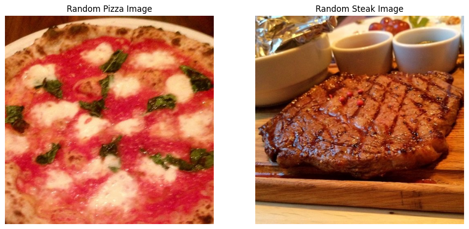
# display random images
def view_random_image(target_dir, target_class):
    target_folder = str(target_dir) + "/" + target_class
    random_image = random.sample(os.listdir(target_folder), 1)
    
    img = mpimg.imread(target_folder + "/" + random_image[0])
    plt.imshow(img)
    plt.title(str(target_class) + str(img.shape))
    plt.axis("off")
    
    return tf.constant(img)

fig = plt.figure(figsize=(12, 12))
plot1 = fig.add_subplot(1, 2, 1)
pizza_image = view_random_image(target_dir = training_data_dir, target_class=class_names[0])
plot2 = fig.add_subplot(1, 2, 2)
steak_image = view_random_image(target_dir = training_data_dir, target_class=class_names[1])
plot1.title.set_text('Random Pizza Image')
plot2.title.set_text('Random Steak Image')

sample_image / 255

# the image is 512x384 pixels with 3 colour values per pixel
# to normalize the rgb values we need to divide all by 255

# <tf.Tensor: shape=(382, 512, 3), dtype=float32, numpy=
# array([[[0.8156863 , 0.7294118 , 0.87058824],
#         [0.827451  , 0.73333335, 0.8666667 ],
#         [0.8392157 , 0.73333335, 0.87058824],
#         ...,
#        [[0.75686276, 0.5254902 , 0.3529412 ],
#         [0.7411765 , 0.50980395, 0.3372549 ],
#         [0.7176471 , 0.4745098 , 0.3137255 ],
#         ...,
#         [0.59607846, 0.49803922, 0.38039216],
#         [0.6431373 , 0.5372549 , 0.42352942],
#         [0.65882355, 0.5529412 , 0.43529412]]], dtype=float32)>

Building the Model

In machine learning, a classifier assigns a class label to a data point. For example, an image classifier produces a class label (e.g, pizza, steak) for what objects exist within an image. A convolutional neural network, or CNN for short, is a type of classifier, which excels at solving this problem.

Rebuilding the Tiny VGG Architecture

(see CNN Explainer)

• Preprocessing:

tf.keras.utils.image_dataset_from_directory(
    directory,
    labels='inferred',
    label_mode='int',
    class_names=None,
    color_mode='rgb',
    batch_size=32,
    image_size=(256, 256),
    shuffle=True,
    seed=None,
    validation_split=None,
    subset=None,
    interpolation='bilinear',
    follow_links=False,
    crop_to_aspect_ratio=False,
    **kwargs
)

• If labels is inferred", the directory should contain subdirectories, each containing images for a class. Otherwise, the directory structure is ignored. "inferred" (labels are generated from the directory structure), None (no labels), or a list/tuple of integer labels of the same size as the number of image files found in the directory. Labels should be sorted according to the alphanumeric order of the image file paths
• String describing the encoding of labels. Options are:
  • int: means that the labels are encoded as integers (e.g. for sparse_categorical_crossentropy loss).
  • categorical: means that the labels are encoded as a categorical vector (e.g. for categorical_crossentropy loss).
  • binary means that the labels (there can be only 2) are encoded as float32 scalars with values 0 or 1 (e.g. for binary_crossentropy).
  • None (no labels).

Conv2D Layer Options

• Filters: How many filters should be applied to the input tensor (10, 32, 64, 128).
• Kernel Size: Sets the filter size.
• Padding: same pads target tensor with zeros to preserve input shape. valid lowers the output shape.
• Strides: strides=1 moves the filter across an image 1 pixel at a time.

seed = 42
batch_size = 32
img_height = 224
img_width = 224

tf.random.set_seed(seed)

# train and test data dirs
train_dir = "../datasets/pizza_steak/train/"
test_dir = "../datasets/pizza_steak/test/"

training_data = image_dataset_from_directory(train_dir,
                                              labels='inferred',
                                              label_mode='binary',
                                              seed=seed,
                                              image_size=(img_height, img_width),
                                              batch_size=batch_size)

testing_data = image_dataset_from_directory(test_dir,
                                              labels='inferred',
                                              label_mode='binary',
                                              seed=seed,
                                              image_size=(img_height, img_width),
                                              batch_size=batch_size)

# building the model
cnn_model = Sequential([
  Rescaling(1./255),
  Conv2D(filters=10, 
         kernel_size=3,
         activation="relu", 
         input_shape=(224, 224, 3)),
  Conv2D(10, 3, activation="relu"),
  MaxPool2D(pool_size=2, padding="same"),
  Conv2D(10, 3, activation="relu"),
  Conv2D(10, 3, activation="relu"),
  MaxPool2D(2),
  Flatten(),
  Dense(1, activation="sigmoid")
])

# compile the model
cnn_model.compile(loss="binary_crossentropy",
                 optimizer=Adam(learning_rate=1e-3),
                 metrics=["accuracy"])

# fitting the model
history_cnn = cnn_model.fit(training_data, epochs=5,
                            steps_per_epoch=len(training_data),
                            validation_data=testing_data,
                            validation_steps=len(testing_data))

# Found 1500 images belonging to 2 classes.
# Found 500 images belonging to 2 classes.
# Epoch 1/5

# Epoch 5/5
# 47/47 [==============================] - 2s 47ms/step - loss: 0.3347 - accuracy: 0.8540 - val_loss: 0.2927 - val_accuracy: 0.8820

cnn_model.summary()

# Model: "sequential_8"
# _________________________________________________________________
#  Layer (type)                Output Shape              Param #   
# =================================================================
#  rescaling (Rescaling)       (None, 224, 224, 3)       0 
#  conv2d_35 (Conv2D)          (None, 222, 222, 10)      280 
#  conv2d_36 (Conv2D)          (None, 220, 220, 10)      910 
#  max_pooling2d_17 (MaxPooling2D)  (None, 110, 110, 10) 0 
#  conv2d_37 (Conv2D)          (None, 108, 108, 10)      910 
#  conv2d_38 (Conv2D)          (None, 106, 106, 10)      910
#  max_pooling2d_18 (MaxPooling2D)  (None, 53, 53, 10)   0
#  flatten_8 (Flatten)         (None, 28090)             0
#  dense_8 (Dense)             (None, 1)                 28091 
# =================================================================
# Total params: 31,101
# Trainable params: 31,101
# Non-trainable params: 0
# _________________________________________________________________

Building a Baseline Model

Above I already started with a CNN that was ideal for the given problem. Let's take a few steps back and try to work our way up to it by establishing a simple and fast baseline first. Fitting a machine learning model follows 3 steps:

1. Create a Baseline Model
2. Overfit a complexer model to improve the validation metric

• Increase # of conv layers
• Increas # of filters in conv layers
• Add another dense layer above the output

3. Reduce the overfit

• Add data augmentation
• Add regularization layers (like pooling layers)
• Add more, varied training data

tf.random.set_seed(42)

model_cnn_base = Sequential([
  Rescaling(1./255),
  Conv2D(filters=10,
          kernel_size=(3, 3),
          strides=(1, 1),
          padding="same",
          activation="relu",
          input_shape=(224, 224, 3),
          name="input_layer"),
  Conv2D(10, 3, activation="relu"),
  Conv2D(10, 3, activation="relu"),
  Flatten(),
  Dense(1, activation="sigmoid", name="output_layer")
])

model_cnn_base.compile(loss="binary_crossentropy",
                      optimizer=Adam(learning_rate=(1e-3)),
                      metrics=["accuracy"])

history_cnn_baseline = model_cnn_base.fit(training_data, epochs=5,
                        steps_per_epoch=len(training_data),
                        validation_data=testing_data,
                        validation_steps=len(testing_data))

# Epoch 5/5
# 47/47 [==============================] - 3s 59ms/step - loss: 0.0901 - accuracy: 0.9740 - val_loss: 0.4827 - val_accuracy: 0.8020

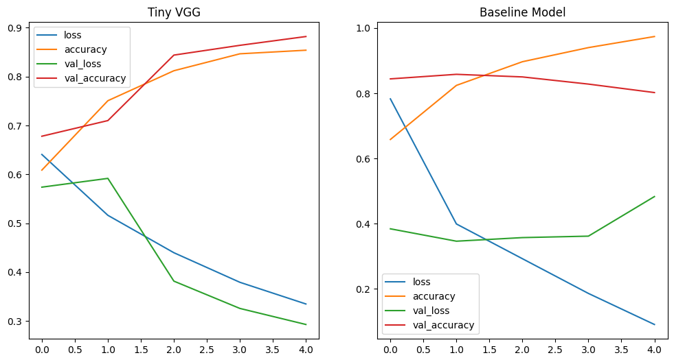
Evaluating the Baseline Model

# print loss curves
fig, axes = plt.subplots(nrows=1, ncols=2, figsize=(12, 6))
pd.DataFrame(history_cnn.history).plot(ax=axes[0], title="Tiny VGG")
pd.DataFrame(history_cnn_baseline.history).plot(ax=axes[1], title="Baseline Model")

# as pointed out above - we can see that the validation loss for the baseline model
# stops improving. But the loss on the trainings data keeps falling
# => this points to our model __overfitting__ the training dataset

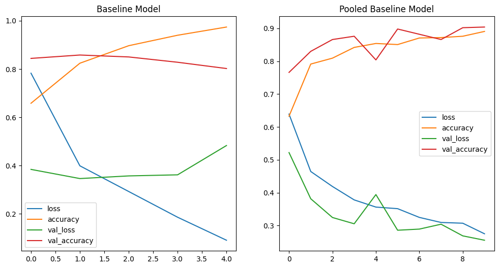
Reducing the Overfit

Improve the evaluation metrics by tackling the overfitting issue:

# adding pooling layers
# maxpool takes a square with size=poolsize (2 => 2x2)
# combines those pixel into 1 with the max value
# this looses fine details and directs your model
# towards the larger features in your image
model_cnn_base_pool = Sequential([
    Rescaling(1./255),
    Conv2D(10, 3, activation="relu", input_shape=(224, 224, 3)),
    MaxPool2D(pool_size=2),
    Conv2D(10, 2, activation="relu"),
    MaxPool2D(),
    Conv2D(10, 2, activation="relu"),
    MaxPool2D(),
    Flatten(),
    Dense(1, activation="sigmoid")
])

model_cnn_base_pool.compile(loss="binary_crossentropy",
                           optimizer=Adam(learning_rate=1e-3),
                           metrics=["accuracy"])

history_cnn_baseline_pool = model_cnn_base_pool.fit(training_data, epochs=10,
                        steps_per_epoch=len(training_data),
                        validation_data=testing_data,
                        validation_steps=len(testing_data))

# Epoch 10/10
# 47/47 [==============================] - 1s 27ms/step - loss: 0.2748 - accuracy: 0.8907 - val_loss: 0.2552 - val_accuracy: 0.9040

# print loss curves
fig, axes = plt.subplots(nrows=1, ncols=2, figsize=(12, 6))
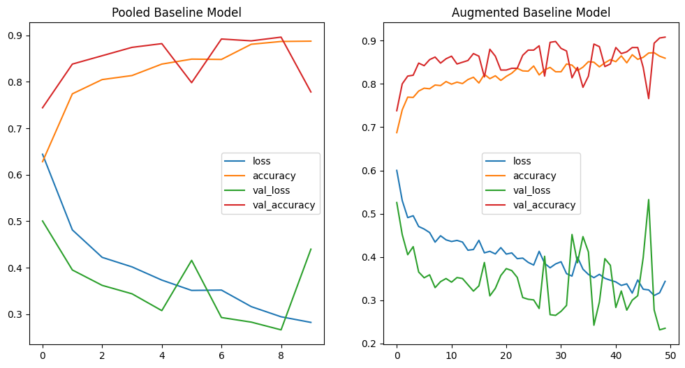
pd.DataFrame(history_cnn_baseline.history).plot(ax=axes[0], title="Baseline Model")
pd.DataFrame(history_cnn_baseline_pool.history).plot(ax=axes[1], title="Pooled Baseline Model")

# I increased the number of epochs to better see the result
# now it is obvious - adding pooling layers already solved the overfit

Another tool we can use to improve the performance of an overfitting model is Data Augmentation.

# to further generalize we could add more images that add variations
# but we get a similar effect from just modifying our training images
# randomly using augmentations to increase diversity

data_augmentation = Sequential([
    RandomFlip("horizontal_and_vertical"),
    RandomRotation(0.2),
    RandomZoom(0.1),
    RandomContrast(0.2),
    RandomBrightness(factor=0.2)
])

model_cnn_base_pool_aug = Sequential([
    data_augmentation,
    Rescaling(1./255),
    Conv2D(10, 3, activation="relu", input_shape=(224, 224, 3)),
    MaxPool2D(pool_size=2),
    Conv2D(10, 2, activation="relu"),
    MaxPool2D(),
    Conv2D(10, 2, activation="relu"),
    MaxPool2D(),
    Flatten(),
    Dense(1, activation="sigmoid")
])

model_cnn_base_pool_aug.compile(loss="binary_crossentropy",
                           optimizer=Adam(learning_rate=1e-3),
                           metrics=["accuracy"])

history_cnn_baseline_pool_aug = model_cnn_base_pool_aug.fit(training_data, epochs=50,
                        steps_per_epoch=len(training_data),
                        validation_data=testing_data,
                        validation_steps=len(testing_data))

# Epoch 50/50
# 47/47 [==============================] - 7s 145ms/step - loss: 0.3436 - accuracy: 0.8593 - val_loss: 0.2353 - val_accuracy: 0.9080

# print loss curves
fig, axes = plt.subplots(nrows=1, ncols=2, figsize=(12, 6))
pd.DataFrame(history_cnn_baseline_pool.history).plot(ax=axes[0], title="Pooled Baseline Model")
pd.DataFrame(history_cnn_baseline_pool_aug.history).plot(ax=axes[1], title="Augmented Baseline Model")

# adding too many data augmentation can lead to a degradation of the performance of a model

Add shuffle to our datasets:

# randomize the order in which your models see the training images
# to remove biases in the order the data was collected in
seed = 42
batch_size = 32
img_height = 224
img_width = 224

tf.random.set_seed(seed)

# train and test data dirs
train_dir = "../datasets/pizza_steak/train/"
test_dir = "../datasets/pizza_steak/test/"

training_data_shuffled = image_dataset_from_directory(train_dir,
                                              labels='inferred',
                                              label_mode='binary',
                                              seed=seed,
                                              shuffle=True,
                                              image_size=(img_height, img_width),
                                              batch_size=batch_size)

testing_data_shuffled = image_dataset_from_directory(test_dir,
                                              labels='inferred',
                                              label_mode='binary',
                                              seed=seed,
                                              shuffle=True,
                                              image_size=(img_height, img_width),
                                              batch_size=batch_size)

# Found 1500 files belonging to 2 classes.
# Found 500 files belonging to 2 classes.

# re-run the same pooled and augmented model as before on shuffled data
data_augmentation = Sequential([
    RandomFlip("horizontal_and_vertical"),
    RandomRotation(0.2),
    RandomZoom(0.1),
    RandomContrast(0.2),
    RandomBrightness(factor=0.2)
])

model_cnn_base_pool_aug_shuffle = Sequential([
    data_augmentation,
    Rescaling(1./255),
    Conv2D(10, 3, activation="relu", input_shape=(224, 224, 3)),
    MaxPool2D(pool_size=2),
    Conv2D(10, 2, activation="relu"),
    MaxPool2D(),
    Conv2D(10, 2, activation="relu"),
    MaxPool2D(),
    Flatten(),
    Dense(1, activation="sigmoid")
])

model_cnn_base_pool_aug_shuffle.compile(loss="binary_crossentropy",
                           optimizer=Adam(learning_rate=1e-3),
                           metrics=["accuracy"])

history_cnn_baseline_pool_aug_shuffle = model_cnn_base_pool_aug_shuffle.fit(training_data_shuffled, epochs=50,
                        steps_per_epoch=len(training_data_shuffled),
                        validation_data=testing_data_shuffled,
                        validation_steps=len(testing_data_shuffled))

# Epoch 50/50
# 47/47 [==============================] - 8s 160ms/step - loss: 0.3257 - accuracy: 0.8580 - val_loss: 0.2617 - val_accuracy: 0.8860

# print loss curves
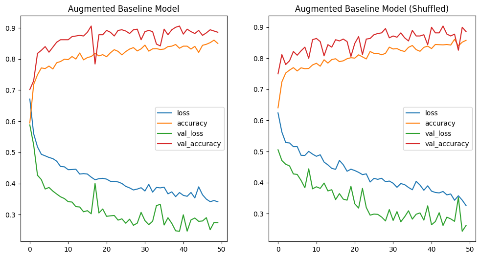
fig, axes = plt.subplots(nrows=1, ncols=2, figsize=(12, 6))
pd.DataFrame(history_cnn_baseline_pool_aug.history).plot(ax=axes[0], title="Augmented Baseline Model")
pd.DataFrame(history_cnn_baseline_pool_aug_shuffle.history).plot(ax=axes[1], title="Augmented Baseline Model (Shuffled)")

# the shuffled data shows a much steeper descent in the loss value:

fig, axes = plt.subplots(nrows=1, ncols=2, figsize=(12, 6))
pd.DataFrame(history_cnn.history).plot(ax=axes[0], title="Original Tiny VGG")
pd.DataFrame(history_cnn_baseline_pool_aug_shuffle.history).plot(ax=axes[1], title="Augmented Baseline Model (Shuffled)")

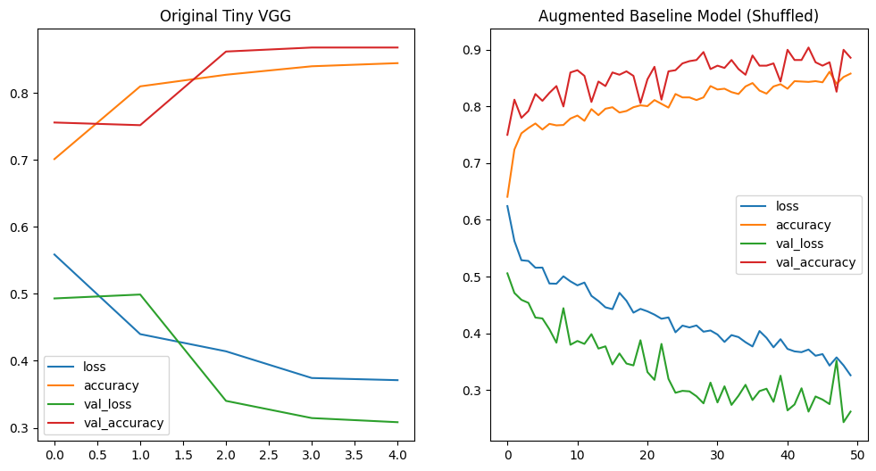
Now that I have the data preprocessing dialed and am getting similar results to the initial Tiny VGG run I want to see how this model performce now with the optimized data:

# re-run the augmented data through the Tiny VGG architecture model
data_augmentation = Sequential([
    RandomFlip("horizontal_and_vertical"),
    RandomRotation(0.2),
    RandomZoom(0.1),
    RandomContrast(0.2),
    RandomBrightness(factor=0.2)
])

vgg_model = Sequential([
  data_augmentation,
  Rescaling(1./255),
  Conv2D(filters=10, 
         kernel_size=3,
         activation="relu", 
         input_shape=(224, 224, 3)),
  Conv2D(10, 3, activation="relu"),
  MaxPool2D(pool_size=2, padding="same"),
  Conv2D(10, 3, activation="relu"),
  Conv2D(10, 3, activation="relu"),
  MaxPool2D(2),
  Flatten(),
  Dense(1, activation="sigmoid")
])

vgg_model.compile(loss="binary_crossentropy",
                           optimizer=Adam(learning_rate=1e-3),
                           metrics=["accuracy"])

history_vgg_model = vgg_model.fit(training_data_shuffled, epochs=50,
                        steps_per_epoch=len(training_data_shuffled),
                        validation_data=testing_data_shuffled,
                        validation_steps=len(testing_data_shuffled))

# Epoch 50/50
# 47/47 [==============================] - 8s 175ms/step - loss: 0.2746 - accuracy: 0.8927 - val_loss: 0.2192 - val_accuracy: 0.9200

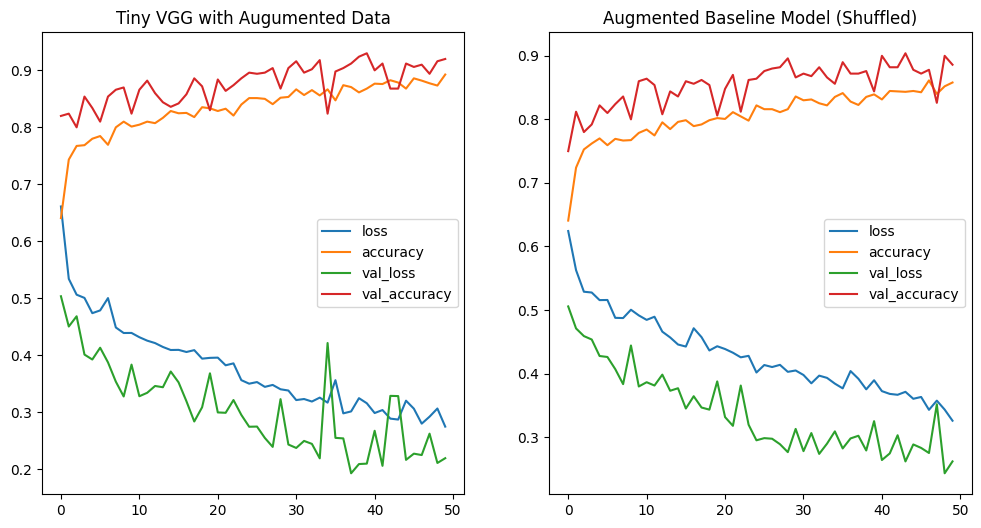
fig, axes = plt.subplots(nrows=1, ncols=2, figsize=(12, 6))
pd.DataFrame(history_cnn_baseline_pool_aug_shuffle.history).plot(ax=axes[1], title="Augmented Baseline Model (Shuffled)")
pd.DataFrame(history_vgg_model.history).plot(ax=axes[0], title="Tiny VGG with Augumented Data")

Making Predictions on Custom Data

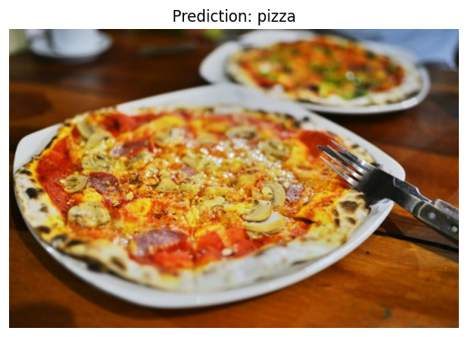
Now that I have a model that looks like it is performing well I can try to run a prediction on a personal picture from my favorite pizza place on the beach of Koh Rong in Cambodia:

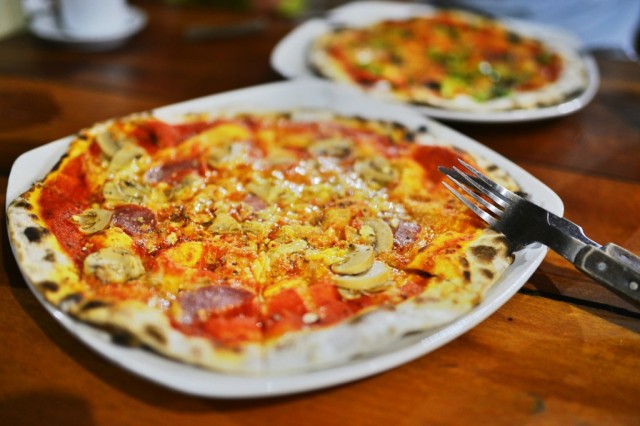
pizza_path = "../assets/pizza.jpg"
pizza_img = mpimg.imread(pizza_path)
pizza_img.shape
# (426, 640, 3)
# before passing the image to our model we first need to pre-process it the same
# way we processed our training images.

steak_path = "../assets/steak.jpg"

# helper function to pre-process images for predictions
def prepare_image(file_name, im_shape=224):
    # read in image
    img = tf.io.read_file(file_name)
    # image array => tensor
    img = tf.image.decode_image(img)
    # reshape to training size
    img = tf.image.resize(img, size=[im_shape, im_shape])
    # we don't need to normalize the image this is done by the model itself
    # img = img/255
    # add a dimension in front for batch size => shape=(1, 224, 224, 3)
    img = tf.expand_dims(img, axis=0)
    return img

test_image_steak = prepare_image(file_name=steak_path)
test_image_pizza = prepare_image(file_name=pizza_path)
test_image_pizza
# the image now has the right shape to be ingested by our model:
# <tf.Tensor: shape=(1, 224, 224, 3), dtype=float32, numpy=
# array([[[[136.07143  , 141.07143  , 111.07143  ],
#          ...

prediction_pizza = vgg_model.predict(test_image_pizza)
prediction_pizza
# we receive a prediction probability of `~0.86`
# array([[0.02831189]], dtype=float32)

# make the propability output "readable"
pred_class_pizza = class_names[int(tf.round(prediction_pizza))]
pred_class_pizza
# 'pizza'

prediction_steak = vgg_model.predict(test_image_steak)
pred_class_steak = class_names[int(tf.round(prediction_steak))]
pred_class_steak
# 'steak'

# making the process a bit more visually appealing
def predict_and_plot(model, file_name, class_names):
    # load the image and preprocess
    img = prepare_image(file_name)
    # run prediction
    prediction = model.predict(img)
    # get predicted class name
    pred_class = class_names[int(tf.round(prediction))]
    # plot image & prediction
    plt.imshow(mpimg.imread(file_name))
    plt.title(f"Prediction: {pred_class}")
    plt.axis(False)

# a few more images to test with
pizza_path2 = "../assets/pizza2.jpg"
pizza_path3 = "../assets/pizza3.jpg"
steak_path2 = "../assets/steak2.jpg"
steak_path3 = "../assets/steak3.jpg"

predict_and_plot(model=vgg_model, file_name=pizza_path3, class_names=class_names)