Tensorflow Representation Learning

Auto encoders are a type of Artificial Neural Networks (ANN) that are used to perform data encoding (Representation Learning). Auto encoder use the same data for input data and output data:
- Feed Forward ANN (Supervised Learning):
- Cat Image
=>ANN<=True Label (Cat)
- Cat Image
- Auto Encoder ANN (Unsupervised Learning):
- Cat Image
=>Encoder ANN/Decoder ANN=>Reconstructed Cat Image=><=Cat Image
- Cat Image
The encoding side of this network generates a representation of the input image (dimensionality reduction). The decoding side then takes the encoded image and tries to reconstruct the input image from it. The performance metric for an Auto Encoder is the similarity between the input and output image.
Denoising Autoencoder
A common use-case for autoencoders is the removal of noise from data, e.g. compression artifacts in low resolution images. This is done by feeding the autoencoder the compressed image and comparing the reconstructed output image to the original, non-compressed image. This training will give us a model that allows us to remove compression artifacts from similarly "mis-treated" images.
Inspecting the Dataset
Start by loading the mnist digits dataset - which is provided by Keras:
# download mnist dataset
from tensorflow.keras.datasets import mnist
(X_train, y_train),(X_test, y_test) = mnist.load_data()
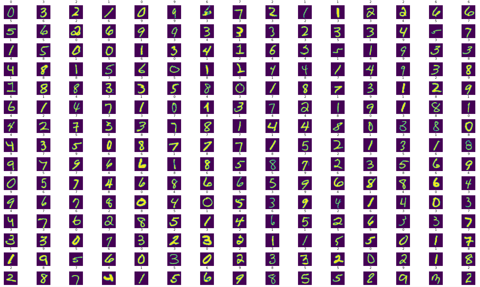
We can inspect a random set of 225 images and their labels from the set using matplotlib:
# inspect a larger set of images
## create a 15x15 grid
W_grid = 15
L_grid = 15
fig, axes = plt.subplots(L_grid, W_grid)
fig, axes = plt.subplots(L_grid, W_grid, figsize = (17,17))
## flaten the 15 x 15 matrix into 225 array
axes = axes.ravel()
## get the length of the training dataset
n_training = len(X_train)

for i in np.arange(0, W_grid * L_grid):
    # select a random number
    index = np.random.randint(0, n_training)
    # read and display an image with the selected index
    axes[i].imshow( X_train[index] )
    axes[i].set_title(y_train[index], fontsize = 8)
    axes[i].axis('off')

plt.subplots_adjust(hspace=0.4)
plt.tight_layout()
plt.show()

Adding Noise
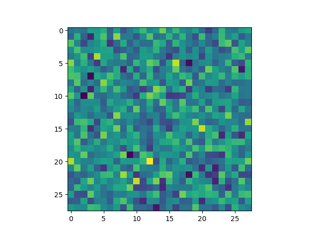
The dataset is clean of noise and can be used as our reference material. To create the "dirty" set of images we can use Numpy to add some random variations:
# create a 28x28 matrix of random number
# added_noise = np.random.randn(*(28,28))
noise_factor = 0.3
added_noise = noise_factor * np.random.randn(*(28,28))

plt.imshow(added_noise)
plt.show()

We can add noise to an existing image the same way:
# adding noise to our image
## how much noise do we need
noise_factor = 0.2
## select an image
sample_image = X_train[666]
## and add noise map to it
noisy_sample_image = sample_image + noise_factor * np.random.randn(*(28,28))

# previs noisy image
plt.imshow(noisy_sample_image, cmap="gray")
plt.show()
Now we can run a loop over both our training and testing dataset, add the same amount of random noise to each image and store those "dirty" datasets in variables:
# add noise to all images in training dataset
X_train_noisy = []
noise_factor = 0.2

for sample_image in X_train:
  sample_image_noisy = sample_image + noise_factor * np.random.randn(*(28,28))
  sample_image_noisy = np.clip(sample_image_noisy, 0., 1.)
  X_train_noisy.append(sample_image_noisy)

# convert list to np array
X_train_noisy = np.array(X_train_noisy)


# add noise to all images in testing dataset
X_test_noisy = []
noise_factor = 0.4

for sample_image in X_test:
  sample_image_noisy = sample_image + noise_factor * np.random.randn(*(28,28))
  sample_image_noisy = np.clip(sample_image_noisy, 0., 1.)
  X_test_noisy.append(sample_image_noisy)

# convert list to np array
X_test_noisy = np.array(X_test_noisy)
Build the Autoencoder
The autoencoder is based on a regular Keras sequential model and consists of the encoder - that is basically the same convolution layer used in regular CNNs with supervised learning - and an decoder - that is an "encoder in reverse". The decoder takes the representation of the image generated by the encoder from the representation layer and has to reconstruct the initial image from this compress data:
# build autoencoder model
autoencoder = tf.keras.models.Sequential()

# build the encoder CNN
autoencoder.add(tf.keras.layers.Conv2D(16, (3,3), strides=1, padding="same", input_shape=(28, 28, 1)))
autoencoder.add(tf.keras.layers.MaxPooling2D((2,2), padding="same"))

autoencoder.add(tf.keras.layers.Conv2D(8, (3,3), strides=1, padding="same"))
autoencoder.add(tf.keras.layers.MaxPooling2D((2,2), padding="same"))

# representation layer
autoencoder.add(tf.keras.layers.Conv2D(8, (3,3), strides=1, padding="same"))

# build the decoder CNN
autoencoder.add(tf.keras.layers.UpSampling2D((2, 2)))
autoencoder.add(tf.keras.layers.Conv2DTranspose(8,(3,3), strides=1, padding="same"))
autoencoder.add(tf.keras.layers.UpSampling2D((2, 2)))
autoencoder.add(tf.keras.layers.Conv2DTranspose(1, (3,3), strides=1, activation='sigmoid', padding="same"))


autoencoder.compile(loss='binary_crossentropy', optimizer=tf.keras.optimizers.Adam(lr=0.001))
autoencoder.summary()
Train the Autoencoder
For the training we now feed the generated noisy dataset into the encoder and have the autencoder compress and reconstruct each image. After those steps we provide to original - noise-free - image to compare the reconstructed image to. The training is complete when we reach a minimum of differences between both of them:
autoencoder.fit(X_train_noisy.reshape(-1, 28, 28, 1),
          X_train.reshape(-1, 28, 28, 1),
          epochs=10,
          batch_size=200)
Evaluate the Model
To get an idea how well our model is performing we can take the first 15 images from the noisy test dataset and compare these source images with the predicted de-noised image:
# test training
# take 15 images from noisy test set and predict de-noised state
denoised_images = autoencoder.predict(X_test_noisy[:15].reshape(-1, 28, 28, 1))
# plot noisy input vs denoised output
fig, axes = plt.subplots(nrows=2, ncols=15, figsize=(30,6))
for images, row in zip([X_test_noisy[:15], denoised_images], axes):
    for img, ax in zip(images, row):
        ax.imshow(img.reshape((28, 28)), cmap='gray')

plt.show()
