Deep Convolutional Generative Adversarial Network

Generative Adversarial Networks (GANs) are one of the most interesting ideas in computer science today. Two models are trained simultaneously by an adversarial process. A Generator ("the artist") learns to create images that look real, while a Discriminator ("the art critic") learns to tell real images apart from fakes.
During training, the generator progressively becomes better at creating images that look real, while the discriminator becomes better at telling them apart. The process reaches equilibrium when the discriminator can no longer distinguish real images from fakes.
Training Dataset
To train the discriminator I am going to use the Fashion mnist dataset provided by Keras:
# configuration
BUFFER_SIZE = 60000
BATCH_SIZE = 256
EPOCHS = 100
noise_dim = 100
num_examples_to_generate = 16
seed = tf.random.normal([num_examples_to_generate, noise_dim])
generator_optimizer = tf.keras.optimizers.Adam(1e-4)
discriminator_optimizer = tf.keras.optimizers.Adam(1e-4)


# import keras fashion mnist fashion dataset (60000 labeled images 28x28)
(train_images, train_labels), (_, _) = tf.keras.datasets.fashion_mnist.load_data()
## preprocess images
# print(rain_images.shape[0])
## 60000
train_images = train_images.reshape(train_images.shape[0], 28, 28, 1).astype('float32')
train_images = (train_images - 127.5) / 127.5 # Normalize the images to [-1, 1]
## batch / shuffle images
train_dataset = tf.data.Dataset.from_tensor_slices(train_images).shuffle(BUFFER_SIZE).batch(BATCH_SIZE)
Fashion-MNIST is a dataset of Zalando's article images—consisting of a training set of 60,000 examples. Each example is a 28x28 grayscale image, associated with a label from 10 classes:
# visualize dataset
plt.imshow(train_images[59999].reshape((28,28)) , cmap = 'gray')
plt.show()
Building the Generator
The Discriminator expects an image as provided by the Fashion mnist dataset - grayscale and with the dimensions 28px times 28px. We can mow build a generator function that based from a random noise seed can generate an image like that:
# build image generator
## the generator should take noise and transform it
## into something the discriminator accepts as a true image

def make_generator_model():
    model = tf.keras.Sequential()
    model.add(layers.Dense(7*7*256, use_bias=False, input_shape=(100,)))
    model.add(layers.BatchNormalization())
    model.add(layers.LeakyReLU())

    model.add(layers.Reshape((7, 7, 256)))

    # Because we used "same" padding and stride = 1, the output is the same size as input 7 x 7 but with 128 filters instead
    model.add(layers.Conv2DTranspose(128, (5, 5), strides=(1, 1), padding='same', use_bias=False))
    model.add(layers.BatchNormalization())
    model.add(layers.LeakyReLU())

    # Because we used "same" padding and stride = 2, the output is double the size of the input 14 x 14 but with 64 filters instead
    model.add(layers.Conv2DTranspose(64, (5, 5), strides=(2, 2), padding='same', use_bias=False))
    model.add(layers.BatchNormalization())
    model.add(layers.LeakyReLU())

    # Because we used "same" padding and stride = 2, the output is double the size of the input 28 x 28 but with 1 filter instead
    model.add(layers.Conv2DTranspose(1, (5, 5), strides=(2, 2), padding='same', use_bias=False, activation='tanh'))
    model.summary()

    return model

generator = make_generator_model()
The final layer outputs an image representation with the dimensions (None, 28, 28, 1):
Model: "sequential"
_________________________________________________________________
 Layer (type)                Output Shape              Param #
=================================================================
 dense (Dense)               (None, 12544)             1254400

 batch_normalization (BatchN  (None, 12544)            50176
 ormalization)

 leaky_re_lu (LeakyReLU)     (None, 12544)             0

 reshape (Reshape)           (None, 7, 7, 256)         0

 conv2d_transpose (Conv2DTra  (None, 7, 7, 128)        819200
 nspose)

 batch_normalization_1 (Batc  (None, 7, 7, 128)        512
 hNormalization)

 leaky_re_lu_1 (LeakyReLU)   (None, 7, 7, 128)         0

 conv2d_transpose_1 (Conv2DT  (None, 14, 14, 64)       204800
 ranspose)

 batch_normalization_2 (Batc  (None, 14, 14, 64)       256
 hNormalization)

 leaky_re_lu_2 (LeakyReLU)   (None, 14, 14, 64)        0

 conv2d_transpose_2 (Conv2DT  (None, 28, 28, 1)        1600
 ranspose)

=================================================================
Total params: 2,330,944
Trainable params: 2,305,472
Non-trainable params: 25,472
_________________________________________________________________
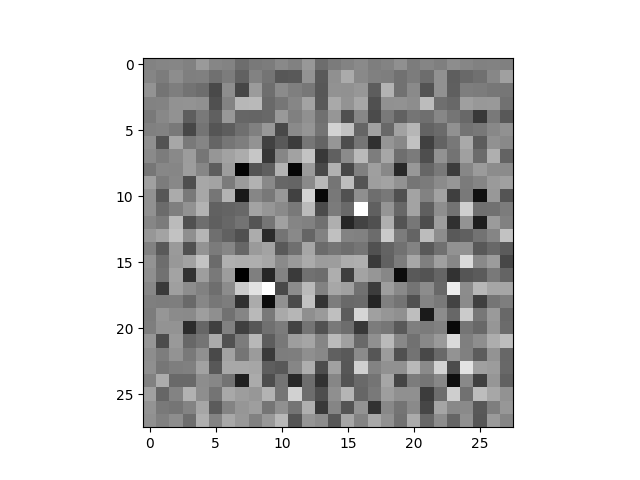
Since we are not yet providing any training the entire function will just take any noise and upscale it to our image dimensions:
# run the generator with a random noise seed
noise = tf.random.normal([1, 100])
generated_image = generator(noise, training=False)
print(generated_image.shape)
plt.imshow(generated_image[0,:,:,0], cmap='gray')
plt.show()
The generated image shape is (1, 28, 28, 1) and is represented by:

Building the Discriminator
Now that we have our generator - that takes in noise and transforms them into whatever we want to train him to do - we can now build the discriminator - who's task it is going to be to evaluate those generated images (or data in general):
# build image discriminator
def make_discriminator_model():
    model = tf.keras.Sequential()
    model.add(layers.Conv2D(64, (5, 5), strides=(2, 2), padding='same', input_shape=[28, 28, 1]))
    model.add(layers.LeakyReLU())
    model.add(layers.Dropout(0.3))

    model.add(layers.Conv2D(128, (5, 5), strides=(2, 2), padding='same'))
    model.add(layers.LeakyReLU())
    model.add(layers.Dropout(0.3))

    model.add(layers.Flatten())
    ## the input image is reduced to a single output
    ## yes/no - how close is this image to a true image
    model.add(layers.Dense(1))
    model.summary()

    return model

discriminator = make_discriminator_model()
Now we can take the generated image from before and let the - yet to be trained - discriminator decide if it is a real image or not:
## feed random seed generated image to discriminator
## the model will have to be trained to output
## positive => real images / negative => detected false
decision = discriminator(generated_image)
print ("Decision: ", decision)
Currently, the output is not yet that helpful. The discriminator decided that the noisy input is 0.00307573 - which means nothing. yet:
Decision: tf.Tensor([[0.00307573]], shape=(1, 1), dtype=float32)
Loss Function
To be able to give feedback on the performance of the prediction model we need a numeric representation of it. For the discriminator training we can compare it's prediction to 1 when the input image was a true image from our training dataset and compare it to 0 for fake, generated images:
# define loss function that calculates the difference
# between a model prediction and the the true label
cross_entropy = tf.keras.losses.BinaryCrossentropy(from_logits=True)

## discriminator loss compares predictions on true images to an array of 1s
## and predictions on generated images to an array of 0s.
def discriminator_loss(real_output, fake_output):
    real_loss = cross_entropy(tf.ones_like(real_output), real_output)
    fake_loss = cross_entropy(tf.zeros_like(fake_output), fake_output)
    total_loss = real_loss + fake_loss # sum up both losses
    return total_loss
During the training Tensorflow will try to minimize this loss - the deviation from the expected value. So that every true image will result in a value close to 1 and every fake one will end up with 0.
So with the discriminator training set we now need to quantify the generator performance. Here the optimum performance is reached when the discriminator judges the generated image to be a true image and assigns it a value close to 1:
## generator loss is low when it's output is judged as a `1` by the discriminator
def generator_loss(fake_output):
    gen_loss = cross_entropy(tf.ones_like(fake_output), fake_output)
    return gen_loss
Model Training
Before running the training we can define Checkpoints that allow us to use the weights generated by an earlier training:
checkpoint_dir = './training_checkpoints'
checkpoint_prefix = os.path.join(checkpoint_dir, "ckpt")
checkpoint = tf.train.Checkpoint(generator_optimizer=generator_optimizer,
                                 discriminator_optimizer=discriminator_optimizer,
                                 generator=generator,
                                 discriminator=discriminator)
Now we can take both the discriminator and generator and train them to minimize their respective loss functions. The training steps are defined as:
## training steps
@tf.function
def train_step(images):
    ## generate random noise as generator input
    noise = tf.random.normal([BATCH_SIZE, noise_dim])

    with tf.GradientTape() as gen_tape, tf.GradientTape() as disc_tape:
      ## call the generator and feed in the noise seed
      generated_images = generator(noise, training=True)
      ## pass the true images to discriminator to perform classification
      real_output = discriminator(images, training=True)
      ## pass the generated images to discriminator to perform classification
      fake_output = discriminator(generated_images, training=True)
      ## generator loss function
      gen_loss = generator_loss(fake_output)
      ## discriminator loss function
      disc_loss = discriminator_loss(real_output, fake_output)

    ## calculate the gradient of the losses
    gradients_of_generator = gen_tape.gradient(gen_loss, generator.trainable_variables)
    gradients_of_discriminator = disc_tape.gradient(disc_loss, discriminator.trainable_variables)
    ## apply the optimizers and update weights
    generator_optimizer.apply_gradients(zip(gradients_of_generator, generator.trainable_variables))
    discriminator_optimizer.apply_gradients(zip(gradients_of_discriminator, discriminator.trainable_variables))
Those steps will be handled by the training function:
## training function
def train(dataset, epochs):
  for epoch in range(epochs):
    start = time.time()

    for image_batch in dataset:
      train_step(image_batch)

    ## save images that are being generated
    display.clear_output(wait=True)
    generate_and_save_images(generator,
                             epoch + 1,
                             seed)

    ## create checkpoint every 15 epochs
    if (epoch + 1) % 15 == 0:
      checkpoint.save(file_prefix = checkpoint_prefix)

    print ('Time for epoch {} is {} sec'.format(epoch + 1, time.time()-start))

  ## generate after the final epoch
  display.clear_output(wait=True)
  generate_and_save_images(generator,
                           epochs,
                           seed)
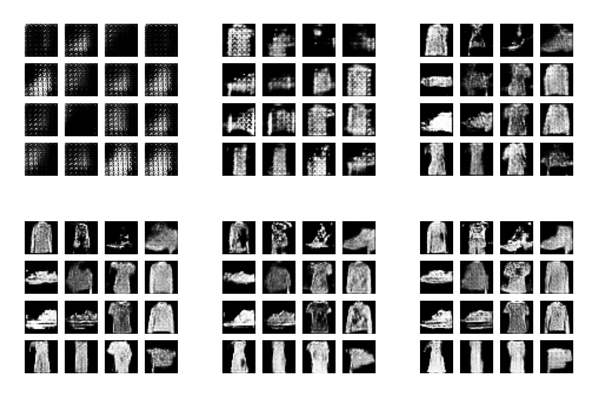
The training function will display the generated images after each epoch and allows us to follow the progress of the training:
## create visual representation of generated images over epochs
def generate_and_save_images(model, epoch, test_input):
  predictions = model(test_input, training=False)

  fig = plt.figure(figsize=(4,4))

  for i in range(predictions.shape[0]):
      plt.subplot(4, 4, i+1)
      plt.imshow(predictions[i, :, :, 0] * 127.5 + 127.5, cmap='gray')
      plt.axis('off')

  plt.savefig('image_at_epoch_{:04d}.png'.format(epoch))
  # plt.show()
