Guangzhou, China

Introduction to Caffe2

Introduction to Caffe2

Setup with Docker

There several images available with and without GPU support - the image tagged latest comes with everything included:

docker pull caffe2ai/caffe2:latest

docker run -it -v /opt/caffe:/home -p 8888:8888 caffe2ai/caffe2:latest jupyter notebook --no-browser --ip=0.0.0.0 --port=8888 --allow-root /home

Make sure that /opt/caffe exists and can be written into by the Docker user.

Copy/paste this URL into your browser when you connect for the first time,
to login with a token: http://0.0.0.0:8888/?token=9346cde0b9a37cda784d193e4e03a18c760847ace645f6cb

You can now access the Jupyter Notebook on your servers IP address on port 8888 with the generated token above.

Testing Installation

Create a new notebook and verify that that Caffe2 is up and running:

from caffe2.python import workspace
import numpy as np
print ("Creating random data")
data = np.random.rand(3, 2)
print(data)
print ("Adding data to workspace ...")
workspace.FeedBlob("mydata", data)
print ("Retrieving data from workspace")
mydata = workspace.FetchBlob("mydata")
print(mydata) 

Introduction to Caffe2

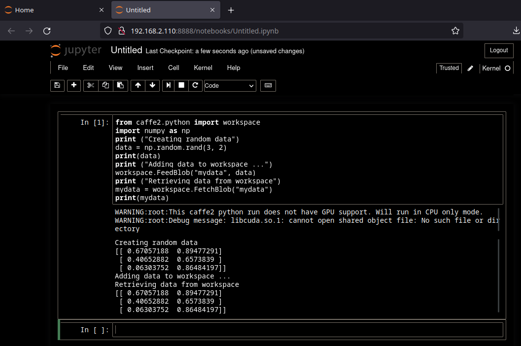
It works!

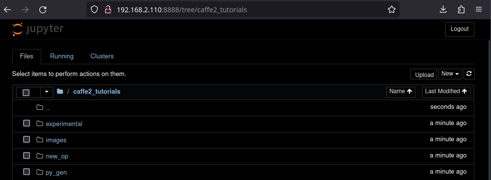
Caffe Tutorial

cd /opt/caffe
git clone --recursive https://github.com/caffe2/tutorials caffe2_tutorials

Introduction to Caffe2

Caffe2 Basic Concepts - Operators & Nets

In this tutorial we will go through a set of Caffe2 basics: the basic concepts including how operators and nets are being written.

First, let's import Caffe2. core and workspace are usually the two that you need most. If you want to manipulate protocol buffers generated by Caffe2, you probably also want to import caffe2_pb2 from caffe2.proto.

from __future__ import absolute_import
from __future__ import division
from __future__ import print_function
from __future__ import unicode_literals

# We'll also import a few standard python libraries
from matplotlib import pyplot
import numpy as np
import time

# These are the droids you are looking for.
from caffe2.python import core, workspace
from caffe2.proto import caffe2_pb2

# Let's show all plots inline.
%matplotlib inline

You might see a warning saying that caffe2 does not have GPU support. That means you are running a CPU-only build. Don't be alarmed - anything CPU is still runnable without a problem.

Workspaces

Let's cover workspaces first, where all the data resides.

Similar to Matlab, the Caffe2 workspace consists of blobs you create and store in memory. For now, consider a blob to be a N-dimensional Tensor similar to numpy's ndarray, but contiguous. Down the road, we will show you that a blob is actually a typed pointer that can store any type of C++ objects, but Tensor is the most common type stored in a blob. Let's show what the interface looks like.

Blobs() prints out all existing blobs in the workspace. HasBlob() queries if a blob exists in the workspace. As of now, we don't have any.

print("Current blobs in the workspace: {}".format(workspace.Blobs()))
print("Workspace has blob 'X'? {}".format(workspace.HasBlob("X")))

We can feed blobs into the workspace using FeedBlob().

X = np.random.randn(2, 3).astype(np.float32)
print("Generated X from numpy:\n{}".format(X))
workspace.FeedBlob("X", X)

Now, let's take a look at what blobs are in the workspace.

print("Current blobs in the workspace: {}".format(workspace.Blobs()))
print("Workspace has blob 'X'? {}".format(workspace.HasBlob("X")))
print("Fetched X:\n{}".format(workspace.FetchBlob("X")))

Let's verify that the arrays are equal.

np.testing.assert_array_equal(X, workspace.FetchBlob("X"))

Note that if you try to access a blob that does not exist, an error will be thrown:

try:
    workspace.FetchBlob("invincible_pink_unicorn")
except RuntimeError as err:
    print(err)

One thing that you might not use immediately: you can have multiple workspaces in Python using different names, and switch between them. Blobs in different workspaces are separate from each other. You can query the current workspace using CurrentWorkspace. Let's try switching the workspace by name (gutentag) and creating a new one if it doesn't exist.

print("Current workspace: {}".format(workspace.CurrentWorkspace()))
print("Current blobs in the workspace: {}".format(workspace.Blobs()))

# Switch the workspace. The second argument "True" means creating 
# the workspace if it is missing.
workspace.SwitchWorkspace("gutentag", True)

# Let's print the current workspace. Note that there is nothing in the
# workspace yet.
print("Current workspace: {}".format(workspace.CurrentWorkspace()))
print("Current blobs in the workspace: {}".format(workspace.Blobs()))

Let's switch back to the default workspace.

workspace.SwitchWorkspace("default")
print("Current workspace: {}".format(workspace.CurrentWorkspace()))
print("Current blobs in the workspace: {}".format(workspace.Blobs()))

Finally, ResetWorkspace() clears anything that is in the current workspace.

workspace.ResetWorkspace()
print("Current blobs in the workspace after reset: {}".format(workspace.Blobs()))

Operators

Operators in Caffe2 are kind of like functions. From the C++ side, they all derive from a common interface, and are registered by type, so that we can call different operators during runtime. The interface of operators is defined in caffe2/proto/caffe2.proto. Basically, it takes in a bunch of inputs, and produces a bunch of outputs.

Remember, when we say "create an operator" in Caffe2 Python, nothing gets run yet. All it does is create the protocol buffer that specifies what the operator should be. At a later time it will be sent to the C++ backend for execution. If you are not familiar with protobuf, it is a json-like serialization tool for structured data. Find more about protocol buffers here.

Let's see an actual example.

# Create an operator.
op = core.CreateOperator(
    "Relu", # The type of operator that we want to run
    ["X"], # A list of input blobs by their names
    ["Y"], # A list of output blobs by their names
)
# and we are done!

As we mentioned, the created op is actually a protobuf object. Let's show the content.

print("Type of the created op is: {}".format(type(op)))
print("Content:\n")
print(str(op))

Ok, let's run the operator. We first feed the input X to the workspace. Then the simplest way to run an operator is to do workspace.RunOperatorOnce(operator)

workspace.FeedBlob("X", np.random.randn(2, 3).astype(np.float32))
workspace.RunOperatorOnce(op)

After execution, let's see if the operator is doing the right thing.

In this case, the operator is a common activation function used in neural networks, called [ReLU](https://en.wikipedia.org/wiki/Rectifier_(neural_networks), or Rectified Linear Unit activation. ReLU activation helps to add necessary non-linear characteristics to the neural network classifier, and is defined as:

$$ReLU(x) = max(0, x)$$

print("Current blobs in the workspace: {}\n".format(workspace.Blobs()))
print("X:\n{}\n".format(workspace.FetchBlob("X")))
print("Y:\n{}\n".format(workspace.FetchBlob("Y")))
print("Expected:\n{}\n".format(np.maximum(workspace.FetchBlob("X"), 0)))

This is working if your Expected output matches your Y output in this example.

Operators also take optional arguments if needed. They are specified as key-value pairs. Let's take a look at one simple example, which takes a tensor and fills it with Gaussian random variables.

op = core.CreateOperator(
    "GaussianFill",
    [], # GaussianFill does not need any parameters.
    ["Z"],
    shape=[100, 100], # shape argument as a list of ints.
    mean=1.0,  # mean as a single float
    std=1.0, # std as a single float
)
print("Content of op:\n")
print(str(op))

Let's run it and see if things are as intended.

workspace.RunOperatorOnce(op)
temp = workspace.FetchBlob("Z")
pyplot.hist(temp.flatten(), bins=50)
pyplot.title("Distribution of Z")

If you see a bell shaped curve then it worked!

Nets

Nets are essentially computation graphs. We keep the name Net for backward consistency (and also to pay tribute to neural nets). A Net is composed of multiple operators just like a program written as a sequence of commands. Let's take a look.

When we talk about nets, we will also talk about BlobReference, which is an object that wraps around a string so we can do easy chaining of operators.

Let's create a network that is essentially the equivalent of the following python math:

X = np.random.randn(2, 3)
W = np.random.randn(5, 3)
b = np.ones(5)
Y = X * W^T + b

We'll show the progress step by step. Caffe2's core.Net is a wrapper class around a NetDef protocol buffer.

When creating a network, its underlying protocol buffer is essentially empty other than the network name. Let's create the net and then show the proto content.

net = core.Net("my_first_net")
print("Current network proto:\n\n{}".format(net.Proto()))

Let's create a blob called X, and use GaussianFill to fill it with some random data.

X = net.GaussianFill([], ["X"], mean=0.0, std=1.0, shape=[2, 3], run_once=0)
print("New network proto:\n\n{}".format(net.Proto()))

You might have observed a few differences from the earlier core.CreateOperator call. Basically, when using a net, you can directly create an operator and add it to the net at the same time by calling net.SomeOp where SomeOp is a registered type string of an operator. This gets translated to:

op = core.CreateOperator("SomeOp", ...)
net.Proto().op.append(op)

Also, you might be wondering what X is. X is a BlobReference which records two things:

The blob's name, which is accessed with str(X)
The net it got created from, which is recorded by the internal variable _from_net

Let's verify it. Also, remember, we are not actually running anything yet, so X contains nothing but a symbol. Don't expect to get any numerical values out of it right now :)

print("Type of X is: {}".format(type(X)))
print("The blob name is: {}".format(str(X)))

Let's continue to create W and b.

W = net.GaussianFill([], ["W"], mean=0.0, std=1.0, shape=[5, 3], run_once=0)
b = net.ConstantFill([], ["b"], shape=[5,], value=1.0, run_once=0)

Now, one simple code sugar: since the BlobReference objects know what net it is generated from, in addition to creating operators from net, you can also create operators from BlobReferences. Let's create the FC operator in this way.

Y = X.FC([W, b], ["Y"])

Under the hood, X.FC(...) simply delegates to net.FC by inserting X as the first input of the corresponding operator, so what we did above is equivalent to

Y = net.FC([X, W, b], ["Y"])

Let's take a look at the current network.

print("Current network proto:\n\n{}".format(net.Proto()))

Too verbose huh? Let's try to visualize it as a graph. Caffe2 ships with a very minimal graph visualization tool for this purpose.

from caffe2.python import net_drawer
from IPython import display
graph = net_drawer.GetPydotGraph(net, rankdir="LR")
display.Image(graph.create_png(), width=800)

So we have defined a Net, but nothing has been executed yet. Remember that the net above is essentially a protobuf that holds the definition of the network. When we actually run the network, what happens under the hood is:

A C++ net object is instantiated from the protobuf
The instantiated net's Run() function is called

Before we do anything, we should clear any earlier workspace variables with ResetWorkspace().

Then there are two ways to run a net from Python. We will do the first option in the example below.

Call workspace.RunNetOnce(), which instantiates, runs and immediately destructs the network
Call workspace.CreateNet() to create the C++ net object owned by the workspace, then call workspace.RunNet(), passing the name of the network to it

workspace.ResetWorkspace()
print("Current blobs in the workspace: {}".format(workspace.Blobs()))
workspace.RunNetOnce(net)
print("Blobs in the workspace after execution: {}".format(workspace.Blobs()))
# Let's dump the contents of the blobs
for name in workspace.Blobs():
    print("{}:\n{}".format(name, workspace.FetchBlob(name)))

Now let's try the second way to create the net, and run it. First, clear the variables with ResetWorkspace(). Then create the net with the workspace's net object that we created earlier using CreateNet(net_object). Finally, run the net with RunNet(net_name).

workspace.ResetWorkspace()
print("Current blobs in the workspace: {}".format(workspace.Blobs()))
workspace.CreateNet(net)
workspace.RunNet(net.Proto().name)
print("Blobs in the workspace after execution: {}".format(workspace.Blobs()))
for name in workspace.Blobs():
    print("{}:\n{}".format(name, workspace.FetchBlob(name)))

There are a few differences between RunNetOnce and RunNet, but the main difference is the computational overhead. Since RunNetOnce involves serializing the protobuf to pass between Python and C and instantiating the network, it may take longer to run. Let's run a test and see what the time overhead is.

# It seems that %timeit magic does not work well with
# C++ extensions so we'll basically do for loops
start = time.time()
for i in range(1000):
    workspace.RunNetOnce(net)
end = time.time()
print('Run time per RunNetOnce: {}'.format((end - start) / 1000))

start = time.time()
for i in range(1000):
    workspace.RunNet(net.Proto().name)
end = time.time()
print('Run time per RunNet: {}'.format((end - start) / 1000))

Congratulations, you now know the many of the key components of the Caffe2 Python API! Ready for more Caffe2? Check out the rest of the tutorials for a variety of interesting use-cases!

Loading Pre-Trained Models

Description

In this tutorial, we will use the pre-trained squeezenet model from the ModelZoo to classify our own images. As input, we will provide the path (or URL) to an image we want to classify. It will also be helpful to know the ImageNet object code for the image so we can verify our results. The 'object code' is nothing more than the integer label for the class used during training, for example "985" is the code for the class "daisy". Note, although we are using squeezenet here, this tutorial serves as a somewhat universal method for running inference on pretrained models.

Note, assuming the last layer of the network is a softmax layer, the results come back as a multidimensional array of probabilities with length equal to the number of classes that the model was trained on. The probabilities may be indexed by the object code (integer type), so if you know the object code you can index the results array at that index to view the network's confidence that the input image is of that class.

Model Download Options

Although we will use squeezenet here, you can check out the Model Zoo for pre-trained models to browse/download a variety of pretrained models, or you can use Caffe2's caffe2.python.models.download module to easily acquire pre-trained models from Github caffe2/models.

For our purposes, we will use the models.download module to download squeezenet into the /caffe2/python/models folder of our local Caffe2 installation with the following command:

python -m caffe2.python.models.download -i squeezenet

Update: The repository has been archived - I am manually downloading this into the container /caffe2/caffe2/python/models/squeezenet:

wget https://github.com/facebookarchive/models/raw/master/squeezenet/init_net.pb
wget https://github.com/facebookarchive/models/raw/master/squeezenet/predict_net.pb
wget https://github.com/facebookarchive/models/raw/master/squeezenet/value_info.json

If the above download worked then you should have a directory named squeezenet in your /caffe2/python/models folder that contains init_net.pb and predict_net.pb. Note, if you do not use the -i flag, the model will be downloaded to your CWD, however it will still be a directory named squeezenet containing two protobuf files. Alternatively, if you wish to download all of the models, you can clone the entire repo using:

git clone https://github.com/caffe2/models

Code

Before we start, lets take care of the required imports.

from __future__ import absolute_import
from __future__ import division
from __future__ import print_function
from __future__ import unicode_literals
%matplotlib inline
from caffe2.proto import caffe2_pb2
import numpy as np
import skimage.io
import skimage.transform
from matplotlib import pyplot
import os
from caffe2.python import core, workspace, models
import urllib2
import operator
print("Required modules imported.")

!mkdir -p /caffe2/caffe2/python/models/squeezenet

!wget https://github.com/facebookarchive/models/raw/master/squeezenet/init_net.pb -P /caffe2/caffe2/python/models/squeezenet
!wget https://github.com/facebookarchive/models/raw/master/squeezenet/predict_net.pb -P /caffe2/caffe2/python/models/squeezenet
!wget https://github.com/facebookarchive/models/raw/master/squeezenet/value_info.json -P /caffe2/caffe2/python/models/squeezenet

!ls -la /caffe2/caffe2/python/models/squeezenet

total 6052
drwxr-xr-x 1 root root      80 Jul 24 06:17 .
drwxr-xr-x 1 root root      20 Jul 24 06:13 ..
-rw-r--r-- 1 root root 6181001 Jul 24 06:15 init_net.pb
-rw-r--r-- 1 root root    6175 Jul 24 06:15 predict_net.pb
-rw-r--r-- 1 root root      32 Jul 24 06:17 value_info.json

Inputs

Here, we will specify the inputs to be used for this run, including the input image, the model location, the mean file (optional), the required size of the image, and the location of the label mapping file.

I downloaded an image flower.jpg and placed it next to the Jupyter Notebook in /opt/caffe/caffe2_tutorials:

# Configuration --- Change to your setup and preferences!
# This directory should contain the models downloaded from the model zoo. To run this 
#   tutorial, make sure there is a 'squeezenet' directory at this location that 
#   contains both the 'init_net.pb' and 'predict_net.pb'
CAFFE_MODELS = "/caffe2/caffe2/python/models"

# Some sample images you can try, or use any URL to a regular image.
IMAGE_LOCATION = "flower.jpg"

# What model are we using?
#    Format below is the model's: <folder, INIT_NET, predict_net, mean, input image size>
#    You can switch 'squeezenet' out with 'bvlc_alexnet', 'bvlc_googlenet' or others that you have downloaded
MODEL = 'squeezenet', 'init_net.pb', 'predict_net.pb', 'ilsvrc_2012_mean.npy', 227

# labels - these help decypher the output and source from a list from ImageNet's object labels 
#    to provide an result like "tabby cat" or "lemon" depending on what's in the picture 
#   you submit to the CNN.
labels =  "https://gist.githubusercontent.com/aaronmarkham/cd3a6b6ac071eca6f7b4a6e40e6038aa/raw/9edb4038a37da6b5a44c3b5bc52e448ff09bfe5b/alexnet_codes"
print("Config set!")

Setup paths

With the configs set, we can now load the mean file (if it exists), as well as the predict net and the init net.

# set paths and variables from model choice and prep image
CAFFE_MODELS = os.path.expanduser(CAFFE_MODELS)

# mean can be 128 or custom based on the model
# gives better results to remove the colors found in all of the training images
MEAN_FILE = os.path.join(CAFFE_MODELS, MODEL[0], MODEL[3])
if not os.path.exists(MEAN_FILE):
    print("No mean file found!")
    mean = 128
else:
    print ("Mean file found!")
    mean = np.load(MEAN_FILE).mean(1).mean(1)
    mean = mean[:, np.newaxis, np.newaxis]
print("mean was set to: ", mean)

# some models were trained with different image sizes, this helps you calibrate your image
INPUT_IMAGE_SIZE = MODEL[4]

# make sure all of the files are around...
INIT_NET = os.path.join(CAFFE_MODELS, MODEL[0], MODEL[1])
PREDICT_NET = os.path.join(CAFFE_MODELS, MODEL[0], MODEL[2])

# Check to see if the files exist
if not os.path.exists(INIT_NET):
    print("WARNING: " + INIT_NET + " not found!")
else:
    if not os.path.exists(PREDICT_NET):
        print("WARNING: " + PREDICT_NET + " not found!")
    else:
        print("All needed files found!")
        

Image Preprocessing

Now that we have our inputs specified and verified the existance of the input network, we can load the image and pre-processing the image for ingestion into a Caffe2 convolutional neural network! This is a very important step as the trained CNN requires a specifically sized input image whose values are from a particular distribution.

# Function to crop the center cropX x cropY pixels from the input image
def crop_center(img,cropx,cropy):
    y,x,c = img.shape
    startx = x//2-(cropx//2)
    starty = y//2-(cropy//2)    
    return img[starty:starty+cropy,startx:startx+cropx]

# Function to rescale the input image to the desired height and/or width. This function will preserve
#   the aspect ratio of the original image while making the image the correct scale so we can retrieve
#   a good center crop. This function is best used with center crop to resize any size input images into
#   specific sized images that our model can use.
def rescale(img, input_height, input_width):
    # Get original aspect ratio
    aspect = img.shape[1]/float(img.shape[0])
    if(aspect>1):
        # landscape orientation - wide image
        res = int(aspect * input_height)
        imgScaled = skimage.transform.resize(img, (input_width, res))
    if(aspect<1):
        # portrait orientation - tall image
        res = int(input_width/aspect)
        imgScaled = skimage.transform.resize(img, (res, input_height))
    if(aspect == 1):
        imgScaled = skimage.transform.resize(img, (input_width, input_height))
    return imgScaled

# Load the image as a 32-bit float
#    Note: skimage.io.imread returns a HWC ordered RGB image of some size
img = skimage.img_as_float(skimage.io.imread(IMAGE_LOCATION)).astype(np.float32)
print("Original Image Shape: " , img.shape)

# Rescale the image to comply with our desired input size. This will not make the image 227x227
#    but it will make either the height or width 227 so we can get the ideal center crop.
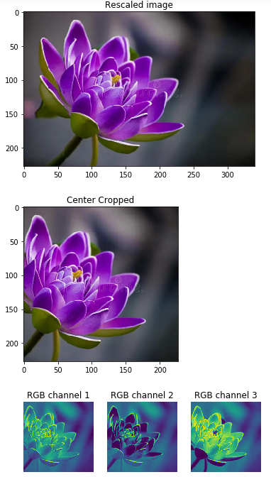
img = rescale(img, INPUT_IMAGE_SIZE, INPUT_IMAGE_SIZE)
print("Image Shape after rescaling: " , img.shape)
pyplot.figure()
pyplot.imshow(img)
pyplot.title('Rescaled image')

# Crop the center 227x227 pixels of the image so we can feed it to our model
img = crop_center(img, INPUT_IMAGE_SIZE, INPUT_IMAGE_SIZE)
print("Image Shape after cropping: " , img.shape)
pyplot.figure()
pyplot.imshow(img)
pyplot.title('Center Cropped')

# switch to CHW (HWC --> CHW)
img = img.swapaxes(1, 2).swapaxes(0, 1)
print("CHW Image Shape: " , img.shape)

pyplot.figure()
for i in range(3):
    # For some reason, pyplot subplot follows Matlab's indexing
    # convention (starting with 1). Well, we'll just follow it...
    pyplot.subplot(1, 3, i+1)
    pyplot.imshow(img[i])
    pyplot.axis('off')
    pyplot.title('RGB channel %d' % (i+1))

# switch to BGR (RGB --> BGR)
img = img[(2, 1, 0), :, :]

# remove mean for better results
img = img * 255 - mean

# add batch size axis which completes the formation of the NCHW shaped input that we want
img = img[np.newaxis, :, :, :].astype(np.float32)

print("NCHW image (ready to be used as input): ", img.shape)

Introduction to Caffe2

Prepare the CNN and run the net!

Now that the image is ready to be ingested by the CNN, let's open the protobufs, load them into the workspace, and run the net.

# Read the contents of the input protobufs into local variables
with open(INIT_NET, "rb") as f:
    init_net = f.read()
with open(PREDICT_NET, "rb") as f:
    predict_net = f.read()

# Initialize the predictor from the input protobufs
p = workspace.Predictor(init_net, predict_net)

# Run the net and return prediction
NCHW_batch = np.zeros((1,3,227,227))
NCHW_batch[0] = img
results = p.run([NCHW_batch.astype(np.float32)])
# Turn it into something we can play with and examine which is in a multi-dimensional array
results = np.asarray(results)
print("results shape: ", results.shape)

# Quick way to get the top-1 prediction result
# Squeeze out the unnecessary axis. This returns a 1-D array of length 1000
preds = np.squeeze(results)
# Get the prediction and the confidence by finding the maximum value and index of maximum value in preds array
curr_pred, curr_conf = max(enumerate(preds), key=operator.itemgetter(1))
print("Prediction: ", curr_pred)
print("Confidence: ", curr_conf)

Prediction: 723
Confidence: 0.910284

Process Results

Recall ImageNet is a 1000 class dataset and observe that it is no coincidence that the third axis of results is length 1000. This axis is holding the probability for each category in the pre-trained model. So when you look at the results array at a specific index, the number can be interpreted as the probability that the input belongs to the class corresponding to that index. Now that we have run the predictor and collected the results, we can interpret them by matching them to their corresponding english labels.

# the rest of this is digging through the results 
results = np.delete(results, 1)
index = 0
highest = 0
arr = np.empty((0,2), dtype=object)
arr[:,0] = int(10)
arr[:,1:] = float(10)
for i, r in enumerate(results):
    # imagenet index begins with 1!
    i=i+1
    arr = np.append(arr, np.array([[i,r]]), axis=0)
    if (r > highest):
        highest = r
        index = i 

# top N results
N = 5
topN = sorted(arr, key=lambda x: x[1], reverse=True)[:N]
print("Raw top {} results: {}".format(N,topN))

# Isolate the indexes of the top-N most likely classes
topN_inds = [int(x[0]) for x in topN]
print("Top {} classes in order: {}".format(N,topN_inds))

# Now we can grab the code list and create a class Look Up Table
response = urllib2.urlopen(labels)
class_LUT = []
for line in response:
    code, result = line.partition(":")[::2]
    code = code.strip()
    result = result.replace("'", "")
    if code.isdigit():
        class_LUT.append(result.split(",")[0][1:])
        
# For each of the top-N results, associate the integer result with an actual class
for n in topN:
    print("Model predicts '{}' with {}% confidence".format(class_LUT[int(n[0])],float("{0:.2f}".format(n[1]*100))))

Raw top 5 results: [array([723.0, 0.9102839827537537], dtype=object), array([968.0, 0.017375782132148743], dtype=object), array([719.0, 0.010471619665622711], dtype=object), array([985.0, 0.009765725582838058], dtype=object), array([767.0, 0.006287392228841782], dtype=object)]

Top 5 classes in order: [723, 968, 719, 985, 767]
- Model predicts: pinwheel with 91.03% confidence
- Model predicts: cup with 1.74% confidence
- Model predicts: piggybank' with 1.05% confidence
- Model predicts: daisy with 0.98% confidence
- Model predicts: rubber eraser with 0.63% confidence

Feeding Larger Batches

Above is an example of how to feed one image at a time. We can achieve higher throughput if we feed multiple images at a time in a single batch. Recall, the data fed into the classifier is in 'NCHW' order, so to feed multiple images, we will expand the 'N' axis.

# List of input images to be fed
images = ["images/cowboy-hat.jpg",
            "images/cell-tower.jpg",
            "images/Ducreux.jpg",
            "images/pretzel.jpg",
            "images/orangutan.jpg",
            "images/aircraft-carrier.jpg",
            "images/cat.jpg"]

# Allocate space for the batch of formatted images
NCHW_batch = np.zeros((len(images),3,227,227))
print ("Batch Shape: ",NCHW_batch.shape)

# For each of the images in the list, format it and place it in the batch
for i,curr_img in enumerate(images):
    img = skimage.img_as_float(skimage.io.imread(curr_img)).astype(np.float32)
    img = rescale(img, 227, 227)
    img = crop_center(img, 227, 227)
    img = img.swapaxes(1, 2).swapaxes(0, 1)
    img = img[(2, 1, 0), :, :]
    img = img * 255 - mean
    NCHW_batch[i] = img

print("NCHW image (ready to be used as input): ", NCHW_batch.shape)

# Run the net on the batch
results = p.run([NCHW_batch.astype(np.float32)])

# Turn it into something we can play with and examine which is in a multi-dimensional array
results = np.asarray(results)

# Squeeze out the unnecessary axis
preds = np.squeeze(results)
print("Squeezed Predictions Shape, with batch size {}: {}".format(len(images),preds.shape))

# Describe the results
for i,pred in enumerate(preds):
    print("Results for: '{}'".format(images[i]))
    # Get the prediction and the confidence by finding the maximum value 
    #   and index of maximum value in preds array
    curr_pred, curr_conf = max(enumerate(pred), key=operator.itemgetter(1))
    print("\tPrediction: ", curr_pred)
    print("\tClass Name: ", class_LUT[int(curr_pred)])
    print("\tConfidence: ", curr_conf)

Batch Shape: (8, 3, 227, 227)
NCHW image (ready to be used as input): (8, 3, 227, 227)
Squeezed Predictions Shape, with batch size 8: (8, 1000)
Results for: 'images/cowboy-hat.jpg'
- Prediction: 515
- Class Name: cowboy hat
- Confidence: 0.850092
Results for: images/cell-tower.jpg
- Prediction: 645
- Class Name: maypole
- Confidence: 0.185843
Results for: images/Ducreux.jpg
- Prediction: 568
- Class Name: fur coat
- Confidence: 0.102531
Results for: images/pretzel.jpg
- Prediction: 932
- Class Name: pretzel
- Confidence: 0.999622
Results for: images/orangutan.jpg
- Prediction: 365
- Class Name: orangutan
- Confidence: 0.992006
Results for: images/aircraft-carrier.jpg
- Prediction: 403
- Class Name: aircraft carrier
- Confidence: 0.999878
Results for: images/cat.jpg
- Prediction: 281
- Class Name: tabby
- Confidence: 0.513315
Results for: images/flower.jpg
- Prediction: 985
- Class Name: daisy
- Confidence: 0.982227

Loading Datasets

So Caffe2 uses a binary DB format to store the data that we would like to train models on. A Caffe2 DB is a glorified name of a key-value storage where the keys are usually randomized so that the batches are approximately i.i.d. The values are the real stuff here: they contain the serialized strings of the specific data formats that you would like your training algorithm to ingest. So, the stored DB would look (semantically) like this:

key1 value1, key2 value2, key3 value3 ...

To a DB, it treats the keys and values as strings, but you probably want structured contents. One way to do this is to use a TensorProtos protocol buffer: it essentially wraps Tensors, aka multi-dimensional arrays, together with the tensor data type and shape information. Then, one can use the TensorProtosDBInput operator to load the data into an SGD training fashion.

Here, we will show you one example of how to create your own dataset. To this end, we will use the UCI Iris dataset - which was a very popular classical dataset for classifying Iris flowers. It contains 4 real-valued features representing the dimensions of the flower, and classifies things into 3 types of Iris flowers. The dataset can be downloaded here.

# First let's import some necessities
from __future__ import absolute_import
from __future__ import division
from __future__ import print_function
from __future__ import unicode_literals

%matplotlib inline
import urllib2 # for downloading the dataset from the web.
import numpy as np
from matplotlib import pyplot
from StringIO import StringIO
from caffe2.python import core, utils, workspace
from caffe2.proto import caffe2_pb2

f = urllib2.urlopen('https://archive.ics.uci.edu/ml/machine-learning-databases/iris/iris.data')
raw_data = f.read()
print('Raw data looks like this:')
print(raw_data[:100] + '...')

Raw data looks like this:
1,3.5,1.4,0.2,Iris-setosa
9,3.0,1.4,0.2,Iris-setosa
7,3.2,1.3,0.2,Iris-setosa
6,3.1,1.5,0.2,...

# load the features to a feature matrix.
features = np.loadtxt(StringIO(raw_data), dtype=np.float32, delimiter=',', usecols=(0, 1, 2, 3))
# load the labels to a feature matrix
label_converter = lambda s : {'Iris-setosa':0, 'Iris-versicolor':1, 'Iris-virginica':2}[s]
labels = np.loadtxt(StringIO(raw_data), dtype=np.int, delimiter=',', usecols=(4,), converters={4: label_converter})

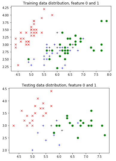
Before we do training, one thing that is often beneficial is to separate the dataset into training and testing. In this case, let's randomly shuffle the data, use the first 100 data points to do training, and the remaining 50 to do testing. For more sophisticated approaches, you can use e.g. cross validation to separate your dataset into multiple training and testing splits. Read more about cross validation here.

random_index = np.random.permutation(150)
features = features[random_index]
labels = labels[random_index]

train_features = features[:100]
train_labels = labels[:100]
test_features = features[100:]
test_labels = labels[100:]

# Let's plot the first two features together with the label.
# Remember, while we are plotting the testing feature distribution
# here too, you might not be supposed to do so in real research,
# because one should not peek into the testing data.
legend = ['rx', 'b+', 'go']
pyplot.title("Training data distribution, feature 0 and 1")
for i in range(3):
    pyplot.plot(train_features[train_labels==i, 0], train_features[train_labels==i, 1], legend[i])
pyplot.figure()
pyplot.title("Testing data distribution, feature 0 and 1")
for i in range(3):
    pyplot.plot(test_features[test_labels==i, 0], test_features[test_labels==i, 1], legend[i])

Introduction to Caffe2

Now, as promised, let's put things into a Caffe2 DB. In this DB, what would happen is that we will use "train_xxx" as the key, and use a TensorProtos object to store two tensors for each data point: one as the feature and one as the label. We will use Caffe2's Python DB interface to do so.

# First, let's see how one can construct a TensorProtos protocol buffer from numpy arrays.
feature_and_label = caffe2_pb2.TensorProtos()
feature_and_label.protos.extend([
    utils.NumpyArrayToCaffe2Tensor(features[0]),
    utils.NumpyArrayToCaffe2Tensor(labels[0])])
print('This is what the tensor proto looks like for a feature and its label:')
print(str(feature_and_label))
print('This is the compact string that gets written into the db:')
print(feature_and_label.SerializeToString())

# Now, actually write the db.

def write_db(db_type, db_name, features, labels):
    db = core.C.create_db(db_type, db_name, core.C.Mode.write)
    transaction = db.new_transaction()
    for i in range(features.shape[0]):
        feature_and_label = caffe2_pb2.TensorProtos()
        feature_and_label.protos.extend([
            utils.NumpyArrayToCaffe2Tensor(features[i]),
            utils.NumpyArrayToCaffe2Tensor(labels[i])])
        transaction.put(
            'train_%03d'.format(i),
            feature_and_label.SerializeToString())
    # Close the transaction, and then close the db.
    del transaction
    del db

write_db("minidb", "iris_train.minidb", train_features, train_labels)
write_db("minidb", "iris_test.minidb", test_features, test_labels)

Now, let's create a very simple network that only consists of one single TensorProtosDBInput operator, to showcase how we load data from the DB that we created. For training, you might want to do something more complex: creating a network, train it, get the model, and run the prediction service. To this end you can look at the MNIST tutorial for details.

net_proto = core.Net("example_reader")
dbreader = net_proto.CreateDB([], "dbreader", db="iris_train.minidb", db_type="minidb")
net_proto.TensorProtosDBInput([dbreader], ["X", "Y"], batch_size=16)

print("The net looks like this:")
print(str(net_proto.Proto()))

workspace.CreateNet(net_proto)

# Let's run it to get batches of features.
workspace.RunNet(net_proto.Proto().name)
print("The first batch of feature is:")
print(workspace.FetchBlob("X"))
print("The first batch of label is:")
print(workspace.FetchBlob("Y"))

# Let's run again.
workspace.RunNet(net_proto.Proto().name)
print("The second batch of feature is:")
print(workspace.FetchBlob("X"))
print("The second batch of label is:")
print(workspace.FetchBlob("Y"))

Image Loading and Preprocessing

In this tutorial we're going to look at how we can load in images from a local file or a URL which you can then utilize in other tutorials or examples. Also, we're going to go in depth on the kinds of preprocessing that is necessary to utilize Caffe2 with images.

from __future__ import absolute_import
from __future__ import division
from __future__ import print_function
from __future__ import unicode_literals

%matplotlib inline
import skimage
import skimage.io as io
import skimage.transform 
import sys
import numpy as np
import math
from matplotlib import pyplot
import matplotlib.image as mpimg
print("Required modules imported.")

Caffe Uses BGR Order

Test an Image
- In the code block below use IMAGE_LOCATION to load what you would like to test. Just change the comment flags to go through each round of the Tutorial. In this way, you'll get to see what happens with a variety of image formats and some tips on how you might preprocess them. If you want to try your own image, drop it in the images folder or use a remote URL. When you pick a remote URL, make it easy on yourself and try to find a URL that points to a common image file type and extension versus some long identifier or query string which might just break this next step.
Color Issues
- Keep in mind when you load images from smartphone cameras that you may run into color formatting issues. Below we show an example of how flipping between RGB and BGR can impact an image. This would obviously throw off detection in your model. Due to legacy support of OpenCV in Caffe and how it handles images in Blue-Green-Red (BGR) order instead of the more commonly used Red-Green-Blue (RGB) order, Caffe2 also expects BGR order. In many ways this decision helps in the long run as you use different computer vision utilities and libraries, but it also can be the source of confusion.

# You can load either local IMAGE_FILE or remote URL
# For Round 1 of this tutorial, try a local image.
IMAGE_LOCATION = 'flower.jpg'

# For Round 2 of this tutorial, try a URL image with a flower: 
# IMAGE_LOCATION = "https://cdn.pixabay.com/photo/2015/02/10/21/28/flower-631765_1280.jpg"
# IMAGE_LOCATION = "images/flower.jpg"

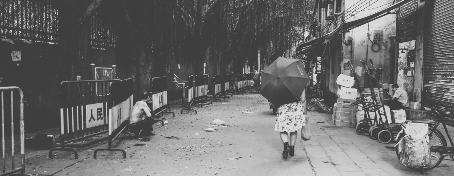
# For Round 3 of this tutorial, try another URL image with lots of people:
# IMAGE_LOCATION = "https://upload.wikimedia.org/wikipedia/commons/1/18/NASA_Astronaut_Group_15.jpg"
# IMAGE_LOCATION = "images/astronauts.jpg"

# For Round 4 of this tutorial, try a URL image with a portrait!
# IMAGE_LOCATION = "https://upload.wikimedia.org/wikipedia/commons/9/9a/Ducreux1.jpg"
# IMAGE_LOCATION = "images/Ducreux.jpg"

img = skimage.img_as_float(skimage.io.imread(IMAGE_LOCATION)).astype(np.float32)

# test color reading
# show the original image
pyplot.figure()
pyplot.subplot(1,2,1)
pyplot.imshow(img)
pyplot.axis('on')
pyplot.title('Original image = RGB')

# show the image in BGR - just doing RGB->BGR temporarily for display
imgBGR = img[:, :, (2, 1, 0)]
#pyplot.figure()
pyplot.subplot(1,2,2)
pyplot.imshow(imgBGR)
pyplot.axis('on')
pyplot.title('OpenCV, Caffe2 = BGR')

Introduction to Caffe2

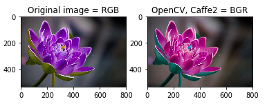
As you can see in the example above, the difference in order is very important to keep in mind. In the code block below we'll be taking the image and converting to BGR order for Caffe to process it appropriately.

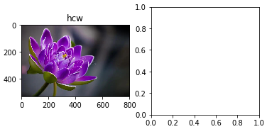
Caffe Prefers CHW Order

H: Height
W: Width
C: Channel (as in color)

Digging even deeper into how image data can be stored is the memory allocation order. You might have noticed when we first loaded the image that we forced it through some interesting transformations. These were data transformations that let us play with the image as if it were a cube. What we see is on top of the cube, and manipulating the layers below can change what we view. We can tinker with it's underlying properties and as you saw above, swap colors quite easily.

For GPU processing, which is what Caffe2 excels at, this order needs to be CHW. For CPU processing, this order is generally HWC. Essentially, you're going to want to use CHW and make sure that step is included in your image pipeline. Tweak RGB to be BGR, which is encapsulated as this "C" payload, then tweak HWC, the "C" being the very same colors you just switched around.

You may ask why! And the reason points to cuDNN which is what helps accelerate processing on GPUs. It uses only CHW, and we'll sum it up by saying it is faster.

img_hcw = "flower.jpg"
img_hcw = skimage.img_as_float(skimage.io.imread(img_hcw)).astype(np.float32)
print("Image shape before HWC --> CHW conversion: ", img_hcw.shape)
# swapping the axes to go from HWC to CHW
# uncomment the next line and run this block!
img_chw = img_hcw.swapaxes(1, 2).swapaxes(0, 1)
print("Image shape after HWC --> CHW conversion: ", img_chw.shape)
# we know this is going to go wrong, so...
try:
    # Plot original
    pyplot.figure()
    pyplot.subplot(1, 2, 1)
    pyplot.imshow(img_hcw)
    pyplot.axis('on')
    pyplot.title('hcw')
    pyplot.subplot(1, 2, 2)
    pyplot.imshow(img_chw)
    pyplot.axis('on')
    pyplot.title('chw')
except:
    print("Here come bad things!")
    # TypeError: Invalid dimensions for image data
    raise 

Introduction to Caffe2

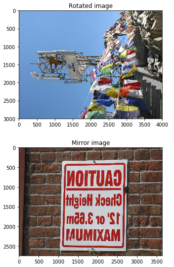
Rotation and Mirroring

This topic is usually reserved for images that are coming from a smart phone. Phones, in general, take great pictures, but do a horrible job communicating how the image was taken and what orientation it should be in. Then there's the user who does everything under the sun with their phone's cameras, making them do things its designer never expected. Cameras - right, because there are often two cameras and these two cameras take different sized pictures in both pixel count and aspect ratio, and not only that, they sometimes take them mirrored, and they sometimes take them in portrait and landscape modes, and sometimes they don't bother to tell which mode they were in.

In many ways this is the first thing you need to evaluate in your pipeline, then look at sizing (described below), then figure out the color situation. If you're developing for iOS, then you're in luck, it's going to be relatively easy. If you're a super-hacker wizard developer with lead-lined shorts and developing for Android, then at least you have lead-lined shorts.

# Image came in sideways - it should be a portait image!
# How you detect this depends on the platform
# Could be a flag from the camera object
# Could be in the EXIF data
# ROTATED_IMAGE = "https://upload.wikimedia.org/wikipedia/commons/8/87/Cell_Phone_Tower_in_Ladakh_India_with_Buddhist_Prayer_Flags.jpg"
ROTATED_IMAGE = "images/cell-tower.jpg"
imgRotated = skimage.img_as_float(skimage.io.imread(ROTATED_IMAGE)).astype(np.float32)
pyplot.figure()
pyplot.imshow(imgRotated)
pyplot.axis('on')
pyplot.title('Rotated image')

# Image came in flipped or mirrored - text is backwards!
# Again detection depends on the platform
# This one is intended to be read by drivers in their rear-view mirror
# MIRROR_IMAGE = "https://upload.wikimedia.org/wikipedia/commons/2/27/Mirror_image_sign_to_be_read_by_drivers_who_are_backing_up_-b.JPG"
MIRROR_IMAGE = "images/mirror-image.jpg"
imgMirror = skimage.img_as_float(skimage.io.imread(MIRROR_IMAGE)).astype(np.float32)
pyplot.figure()
pyplot.imshow(imgMirror)
pyplot.axis('on')
pyplot.title('Mirror image')

Introduction to Caffe2

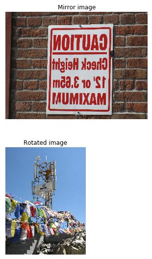
Let's transform these images into something Caffe2 and the standard detection models we have around can detect. Also, this little trick might save you if, say for example, you really had to detect the cell tower but there's no EXIF data to be found: then you'd cycle through every rotation, and every flip, spawning many derivatives of this photo and run them all through. When the percentage of confidence of detection is high enough, Bam!, you found the orientation you needed and that sneaky cell tower.

# Run me to flip the image back and forth
imgMirror = np.fliplr(imgMirror)
pyplot.figure()
pyplot.imshow(imgMirror)
pyplot.axis('off')
pyplot.title('Mirror image')

# Run me to rotate the image 90 degrees
imgRotated = np.rot90(imgRotated, 3)
pyplot.figure()
pyplot.imshow(imgRotated)
pyplot.axis('off')
pyplot.title('Rotated image')

Introduction to Caffe2

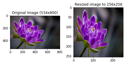
Sizing

Part of preprocessing is resizing. For reasons we won't get into here, images in the Caffe2 pipeline should be square. Also, to help with performance, they should be resized to a standard height and width which is usually going to be smaller than your original source. In the example below we're resizing to 256 x 256 pixels, however you might notice that the input_height and input_width is set to 224 x 224 which is then used to specify the crop. This is what several image-based models are expecting. They were trained on images sized to 224 x 224 and in order for the model to properly identify the suspect images you throw at it, these should also be 224 x 224.

# Model is expecting 224 x 224, so resize/crop needed.
# First, let's resize the image to 256*256
orig_h, orig_w, _ = img.shape
print("Original image's shape is {}x{}".format(orig_h, orig_w))
input_height, input_width = 224, 224
print("Model's input shape is {}x{}".format(input_height, input_width))
img256 = skimage.transform.resize(img, (256, 256))

# Plot original and resized images for comparison
f, axarr = pyplot.subplots(1,2)
axarr[0].imshow(img)
axarr[0].set_title("Original Image (" + str(orig_h) + "x" + str(orig_w) + ")")
axarr[0].axis('on')
axarr[1].imshow(img256)
axarr[1].axis('on')
axarr[1].set_title('Resized image to 256x256')
pyplot.tight_layout()

print("New image shape:" + str(img256.shape))

Original image's shape is 534x800
Model's input shape is 224x224
New image shape:(256, 256, 3)

Introduction to Caffe2

Rescaling

If you imagine portait images versus landscape images you'll know that there are a lot of things that can get messed up by doing a slopping resize. Rescaling is assuming that you're locking down the aspect ratio to prevent distortion in the image. In this case, we'll scale down the image to the shortest side that matches with the model's input size.

Landscape: limit resize by the height
Portrait: limit resize by the width

print("Original image shape:" + str(img.shape) + " and remember it should be in H, W, C!")
print("Model's input shape is {}x{}".format(input_height, input_width))
aspect = img.shape[1]/float(img.shape[0])
print("Orginal aspect ratio: " + str(aspect))
if(aspect>1):
    # landscape orientation - wide image
    res = int(aspect * input_height)
    imgScaled = skimage.transform.resize(img, (input_height, res))
if(aspect<1):
    # portrait orientation - tall image
    res = int(input_width/aspect)
    imgScaled = skimage.transform.resize(img, (res, input_width))
if(aspect == 1):
    imgScaled = skimage.transform.resize(img, (input_height, input_width))
pyplot.figure()
pyplot.imshow(imgScaled)
pyplot.axis('on')
pyplot.title('Rescaled image')
print("New image shape:" + str(imgScaled.shape) + " in HWC")

Original image shape:(534, 800, 3) and remember it should be in H, W, C!
Model's input shape is 224x224
Orginal aspect ratio: 1.49812734082
New image shape:(224, 335, 3) in HWC

At this point only one dimension is set to what the model's input requires. We still need to crop one side to make a square.

Cropping

There are a variety of strategies we could utilize. In fact, we could backpeddle and decide to do a center crop. So instead of scaling down to the smallest we could get on at least one side, we take a chunk out of the middle. If we had done that without scaling we would have ended up with just part of a flower pedal, so we still needed some resizing of the image.

Below we'll try a few strategies for cropping:

Just grab the exact dimensions you need from the middle!
Resize to a square that's pretty close then grab from the middle.
Use the rescaled image and grab the middle.

# Compare the images and cropping strategies
# Try a center crop on the original for giggles
print("Original image shape:" + str(img.shape) + " and remember it should be in H, W, C!")
def crop_center(img,cropx,cropy):
    y,x,c = img.shape
    startx = x//2-(cropx//2)
    starty = y//2-(cropy//2)    
    return img[starty:starty+cropy,startx:startx+cropx]
# yes, the function above should match resize and take a tuple...

pyplot.figure()
# Original image
imgCenter = crop_center(img,224,224)
pyplot.subplot(1,3,1)
pyplot.imshow(imgCenter)
pyplot.axis('on')
pyplot.title('Original')

# Now let's see what this does on the distorted image
img256Center = crop_center(img256,224,224)
pyplot.subplot(1,3,2)
pyplot.imshow(img256Center)
pyplot.axis('on')
pyplot.title('Squeezed')

# Scaled image
imgScaledCenter = crop_center(imgScaled,224,224)
pyplot.subplot(1,3,3)
pyplot.imshow(imgScaledCenter)
pyplot.axis('on')
pyplot.title('Scaled')

pyplot.tight_layout()

Introduction to Caffe2

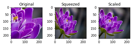
As you can see that didn't work out so well, except for maybe the last one. The middle one may be just fine too, but you won't know until you try on the model and test a lot of candidate images. At this point we can look at the difference we have, split it in half and remove some pixels from each side. This does have a drawback, however, as an off-center subject of interest would get clipped.

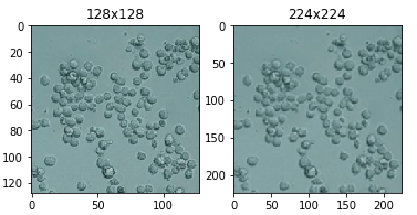
Upscaling

What do you do when the images you want to run are "tiny"? In our example we've been prepping for Input Images with the spec of 224x224. Consider this 128x128 image below.

The most basic approach is going from a small square to a bigger square and using the defauls skimage provides for you. This resize method defaults the interpolation order parameter to 1 which happens to be bi-linear if you even cared, but it is worth mentioning because these might be the fine-tuning knobs you need later to fix problems, such as strange visual artifacts, that can be introduced in upscaling images.

imgTiny = "images/Cellsx128.png"
imgTiny = skimage.img_as_float(skimage.io.imread(imgTiny)).astype(np.float32)
print("Original image shape: ", imgTiny.shape)
imgTiny224 = skimage.transform.resize(imgTiny, (224, 224))
print("Upscaled image shape: ", imgTiny224.shape)
# Plot original
pyplot.figure()
pyplot.subplot(1, 2, 1)
pyplot.imshow(imgTiny)
pyplot.axis('on')
pyplot.title('128x128')
# Plot upscaled
pyplot.subplot(1, 2, 2)
pyplot.imshow(imgTiny224)
pyplot.axis('on')
pyplot.title('224x224')

Original image shape: (128, 128, 4)
Upscaled image shape: (224, 224, 4)

Introduction to Caffe2

Batch Processing

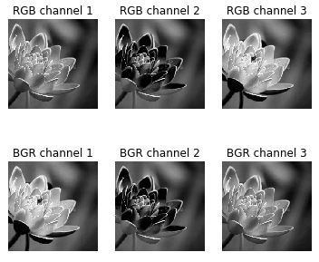
In the last steps below we are going to switch the image's data order to BGR, stuff that into the Color column, then reorder the columns for GPU processing (HCW --> CHW) and then add a fourth dimension (N) to the image to track the number of images. In theory, you can just keep adding dimensions to your data, but this one is required for Caffe2 as it relays to Caffe how many images to expect in this batch. We set it to one (1) to indicate there's only one image going into Caffe in this batch. Note that in the final output when we check img.shape the order is quite different. We've added N for number of images, and changed the order like so: N, C, H, W.

# This next line helps with being able to rerun this section
# if you want to try the outputs of the different crop strategies above
# swap out imgScaled with img (original) or img256 (squeezed)
imgCropped = crop_center(imgScaled,224,224)
print("Image shape before HWC --> CHW conversion: ", imgCropped.shape)
# (1) Since Caffe expects CHW order and the current image is HWC,
#     we will need to change the order.
imgCropped = imgCropped.swapaxes(1, 2).swapaxes(0, 1)
print("Image shape after HWC --> CHW conversion: ", imgCropped.shape)

pyplot.figure()
for i in range(3):
    # For some reason, pyplot subplot follows Matlab's indexing
    # convention (starting with 1). Well, we'll just follow it...
    pyplot.subplot(1, 3, i+1)
    pyplot.imshow(imgCropped[i], cmap=pyplot.cm.gray)
    pyplot.axis('off')
    pyplot.title('RGB channel %d' % (i+1))

# (2) Caffe uses a BGR order due to legacy OpenCV issues, so we
#     will change RGB to BGR.
imgCropped = imgCropped[(2, 1, 0), :, :]
print("Image shape after BGR conversion: ", imgCropped.shape)

# for discussion later - not helpful at this point
# (3) (Optional) We will subtract the mean image. Note that skimage loads
#     image in the [0, 1] range so we multiply the pixel values
#     first to get them into [0, 255].
#mean_file = os.path.join(CAFFE_ROOT, 'python/caffe/imagenet/ilsvrc_2012_mean.npy')
#mean = np.load(mean_file).mean(1).mean(1)
#img = img * 255 - mean[:, np.newaxis, np.newaxis]

pyplot.figure()
for i in range(3):
    # For some reason, pyplot subplot follows Matlab's indexing
    # convention (starting with 1). Well, we'll just follow it...
    pyplot.subplot(1, 3, i+1)
    pyplot.imshow(imgCropped[i], cmap=pyplot.cm.gray)
    pyplot.axis('off')
    pyplot.title('BGR channel %d' % (i+1))
# (4) Finally, since caffe2 expect the input to have a batch term
#     so we can feed in multiple images, we will simply prepend a
#     batch dimension of size 1. Also, we will make sure image is
#     of type np.float32.
imgCropped = imgCropped[np.newaxis, :, :, :].astype(np.float32)
print('Final input shape is:', imgCropped.shape)

Image shape before HWC --> CHW conversion: (224, 224, 3)
Image shape after HWC --> CHW conversion: (3, 224, 224)
Image shape after BGR conversion: (3, 224, 224)
Final input shape is: (1, 3, 224, 224)

Introduction to Caffe2

Introduction to Caffe2

Setup with Docker​

Testing Installation​

Caffe Tutorial​

Caffe2 Basic Concepts - Operators & Nets​

Workspaces​

Operators​

Nets​

Loading Pre-Trained Models​

Description​

Code​

Inputs​

Setup paths​

Image Preprocessing​

Prepare the CNN and run the net!​

Process Results​

Feeding Larger Batches​

Loading Datasets​

Image Loading and Preprocessing​

Caffe Uses BGR Order​

Caffe Prefers CHW Order​

Rotation and Mirroring​

Sizing​

Rescaling​

Cropping​

Upscaling​

Batch Processing​

Setup with Docker

Testing Installation

Caffe Tutorial

Caffe2 Basic Concepts - Operators & Nets

Workspaces

Operators

Nets

Loading Pre-Trained Models

Description

Code

Inputs

Setup paths

Image Preprocessing

Prepare the CNN and run the net!

Process Results

Feeding Larger Batches

Loading Datasets

Image Loading and Preprocessing

Caffe Uses BGR Order

Caffe Prefers CHW Order

Rotation and Mirroring

Sizing

Rescaling

Cropping

Upscaling

Batch Processing