SciKit Wine Quality

• Dataset Exploration
  • Feature Importance
    • Red Wines
    • White Wines
• Data Pre-Processing
  • Binary Classification
  • Data Normalization
  • Data Splitting
• Fitting a Model
  • Decision Tree
  • Random Forest
  • AdaBoost
  • Gradient Boosting
  • XGBoost

Github Repository

Based on Red Wine Quality, Simple and clean practice dataset for regression or classification modelling

Source: The two datasets are related to red and white variants of the Portuguese Vinho Verde wine. For more details, consult the reference Cortez et al., 2009. Due to privacy and logistic issues, only physicochemical (inputs) and sensory (the output) variables are available (e.g. there is no data about grape types, wine brand, wine selling price, etc.).

Dataset Exploration

The quality of a wine is determined by 11 input variables:

• Fixed acidity
• Volatile acidity
• Citric acid
• Residual sugar
• Chlorides
• Free sulfur dioxide
• Total sulfur dioxide
• Density
• pH
• Sulfates
• Alcohol

Start by downloading the dataset:

mkdir data
wget --directory-prefix=data https://archive.ics.uci.edu/ml/machine-learning-databases/wine-quality/winequality.names
wget --directory-prefix=data https://archive.ics.uci.edu/ml/machine-learning-databases/wine-quality/winequality-red.csv
wget --directory-prefix=data https://archive.ics.uci.edu/ml/machine-learning-databases/wine-quality/winequality-white.csv

And take a look at it:

df = pd.read_csv("data/winequality-red.csv")

# See the number of rows and columns
print("Rows, columns: " + str(df.shape))
## Rows, columns: (1599, 1)

# Missing Values
print(df.isna().sum())
# fixed acidity;"volatile acidity";"citric acid";"residual sugar";"chlorides";"free sulfur dioxide";"total sulfur dioxide";"density";"pH";"sulphates";"alcohol";"quality"    0 <- nothing missing
# dtype: int64

# See the first five rows of the dataset
print(df.head())

fixed acidity	volatile acidity	citric acid	residual sugar	chlorides	free sulfur dioxide	total sulfur dioxide	density	pH	sulphates	alcohol	quality
7.4	0.7	0	1.9	0.076	11	34	0.9978	3.51	0.56	9.4	5
7.8	0.88	0	2.6	0.098	25	67	0.9968	3.2	0.68	9.8	5
7.8	0.76	0.04	2.3	0.092	15	54	0.997	3.26	0.65	9.8	5
11.2	0.28	0.56	1.9	0.075	17	60	0.998	3.16	0.58	9.8	6
7.4	0.7	0	1.9	0.076	11	34	0.9978	3.51	0.56	9.4	5

I ran into an issue trying to plot the quality distribution with plotly - I noticed that the source CSV file used ; instead of , to separate cells. Now it works:

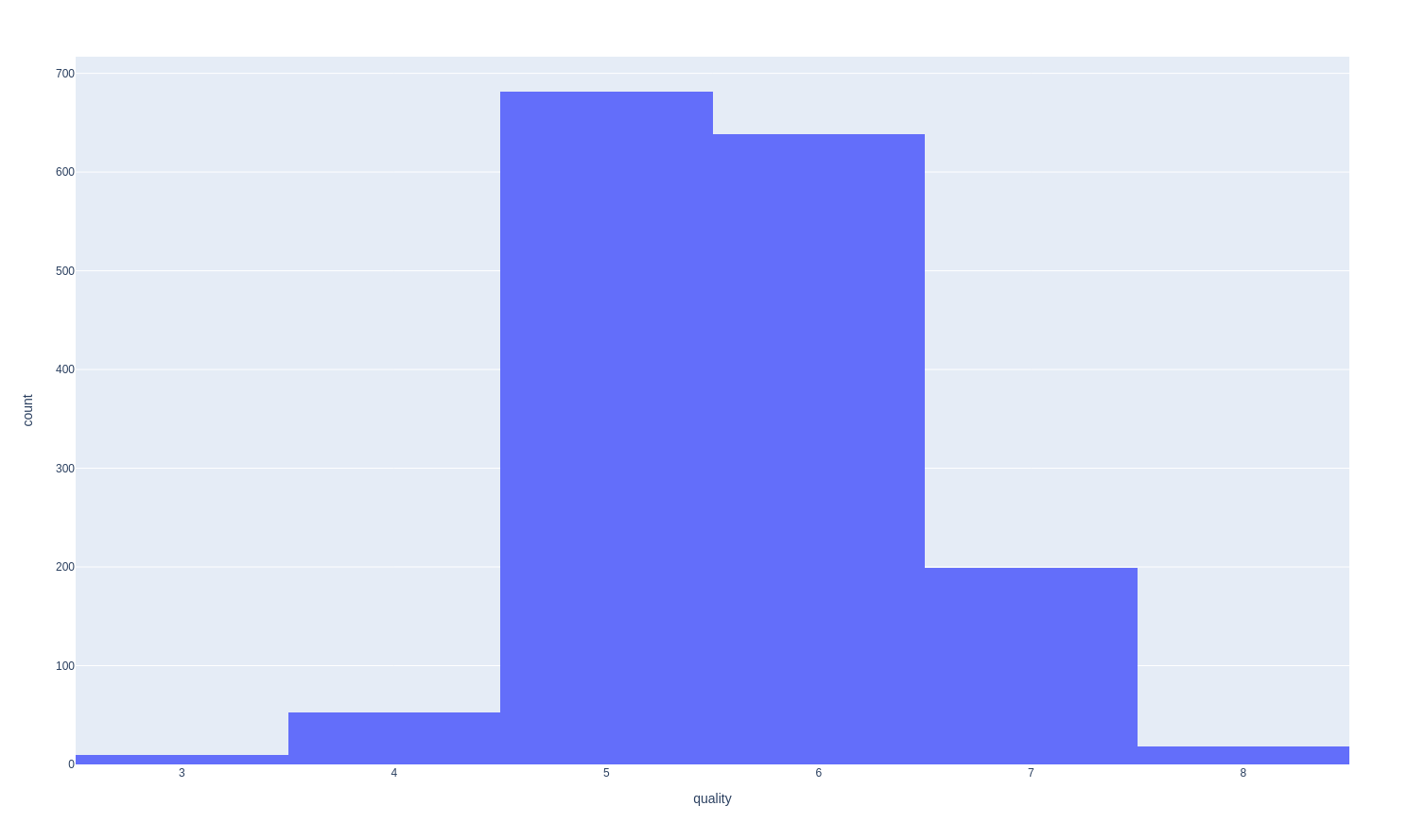
# quality distribution
fig = px.histogram(df,x='quality')
fig.show()

The classes not balanced (e.g. there are much more normal wines than excellent or poor ones):

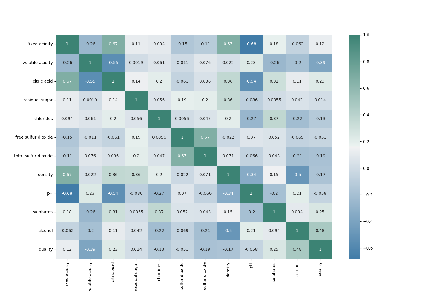
The correlation matrix can show us what labels might have a good correlation with the perceived quality of the wine:

## correlation matrix
corr = df.corr()
plt.subplots(figsize=(15,10))
sns.heatmap(corr, xticklabels=corr.columns, yticklabels=corr.columns, annot=True, cmap=sns.diverging_palette(240, 170, center="light", as_cmap=True))
plt.show()

Feature Importance

The Correlation Matrix already gives us an idea but only after fitting a well performing model can we decide what features are most important when it comes to classifying our wines. SPOILER ALERT: From the 5 classifier I will use below the Random Forrest and XGBoost will have the best performance.

We can use the feature_importances_ function that is provided by the classifiers and extract a ranking of how important is each feature for the resulting classification, sort the results in a Panda Series using nlargest and plot the results.

Red Wines

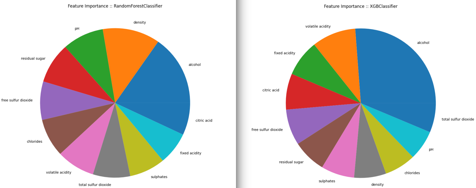
## RandomForestClassifier
feat_importances_forrest = pd.Series(forrest_model.feature_importances_, index=X_features.columns)
feat_importances_forrest.nlargest(11).plot(kind='pie', figsize=(10,10), title="Feature Importance :: RandomForestClassifier")
plt.show()

## XGBClassifier
feat_importances_xbg = pd.Series(xgboost_model.feature_importances_, index=X_features.columns)
feat_importances_xbg.nlargest(11).plot(kind='pie', figsize=(10,10), title="Feature Importance :: XGBClassifier")
plt.show()

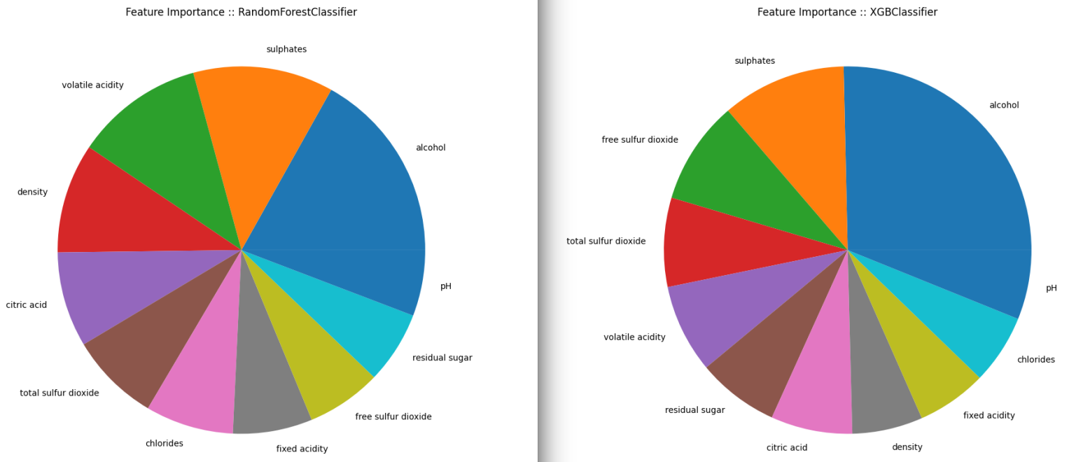
Both classifier models agree that the Alcohol content is the most important factor. Followed by the concentration of Sulphates. But after that their opinions seem to drift apart.

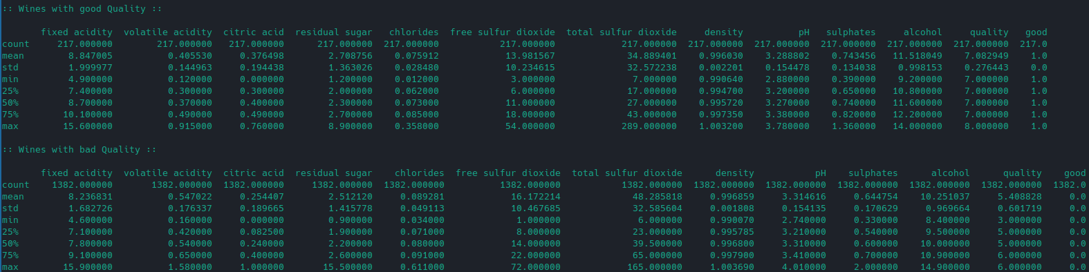
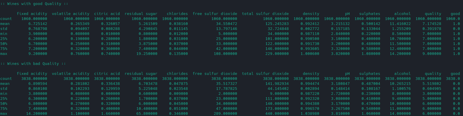
Taking a look at the good and bad wines:

# get only good wines
df_good = df[df['good']==1]
print(":: Wines with good Quality ::")
print("")
print(df_good.describe())
# get only bad wines
df_bad = df[df['good']==0]
print("")
print(":: Wines with bad Quality ::")
print("")
print(df_bad.describe())

We can see that wines that are labelled as being good tend to have a higher alcohol and sulphate concentration:

White Wines

The same analysis for the white wine data shows also emphasizes the importance of the Alcohol content and a balance of sweetness and acidity. The sulfur factor is largely underrepresented:

Data Pre-Processing

And now to the nitty, gritty of actually getting those results. To be able to work with our dataset we first have to do some housecleaning.

Binary Classification

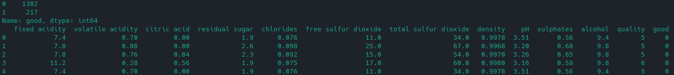
As recommended by the Author we can make quality scale binary - everything with a quality below 7 is just not worth your attention. So let's add another column good and set it's value to 1 if the quality is >= 7 and otherwise to 0:

# make binary quality classification
df['good'] = [1 if x >= 7 else 0 for x in df['quality']]
# separate feature and target variables
X = df.drop(['quality', 'good'], axis = 1)
y = df['good']
# check distribution
print(df['good'].value_counts())
# print first 5 rows
print(df.head())

The result is that we have 217 out of 1599 wines that are worth trying:

Data Normalization

Because all the features in X have different units / scales they cannot be compared directly but need to be normalized. We can use the StandardScaler from SciKit Learn to standardize those features by removing the mean and scaling to unit variance:

# Normalize feature variables
X_features = X
X = StandardScaler().fit_transform(X)

Data Splitting

To train our model we need a training and validation dataset to be able to establish performance metrics. And again it is sklearn with train_test_split that helps us to split the arrays or matrices into random train and test subsets. To get a random 25/75 split we can use:

# Splitting the data
X_train, X_test, y_train, y_test = train_test_split(X, y, test_size=.25, random_state=42)

Fitting a Model

Now we have to find a model that we can fit to our dataset. I found an article by Terence Shin that already explored several solutions to the classification problem.

Decision Tree

Decision Trees are a non-parametric supervised learning method used for classification and regression. The goal is to create a model that predicts the value of a target variable by learning simple decision rules inferred from the data features. A tree can be seen as a piecewise constant approximation.

sklearn provides a A decision tree classifier. that we can apply to our problem

## decision tree classifier
tree_model = DecisionTreeClassifier(random_state=42)
## use training dataset for fitting
tree_model.fit(X_train, y_train)
## run prediction based of the validation dataset
y_pred1 = tree_model.predict(X_test)
## get performance metrics
print(classification_report(y_test, y_pred1))

Running the classifier returns the following - the metrics I am looking out for here are precision and recall that give us a sense for the relation of true and false positives and negatives that were predicted during the validation run:

• precision = TP / (TP + FP) |
• recall = TP / (TP + FN)

	precision	recall	f1-score	support
0	0.94	0.92	0.93	347
1	0.55	0.62	0.58	53
accuracy			0.88	400
macro avg	0.75	0.77	0.76	400
weighted avg	0.89	0.88	0.89	400

We get a reasonably high precision for "bad wines" (0). But it is basically hit or miss for "good wines" (1). Since the dataset is not balanced and weighting in on the bad side we might see a model overfitting here:

• Label 0:
  • PRECISION: Of all wines that were predicted as "not good", 94% were actually labelled with 0.
  • RECALL: Of all wines that were truly labelled 0 we predicted 92% correctly.
• Label 1:
  • PRECISION: Of all wines that were predicted as "good", 55% were actually labelled with 1.
  • RECALL: Of all wines that were truly labelled 1 we predicted 62% correctly.

Random Forest

Next, another sklearn classifier - the RandomForestClassifier. A random forest is a meta estimator that fits a number of decision tree classifiers on various sub-samples of the dataset and uses averaging to improve the predictive accuracy and control over-fitting. The sub-sample size is controlled with the max_samples parameter if bootstrap=True (default), otherwise the whole dataset is used to build each tree:

## random forrest classifier
forrest_model = RandomForestClassifier(random_state=42)
## use training dataset for fitting
forrest_model.fit(X_train, y_train)
## run prediction based of the validation dataset
y_pred2 = forrest_model.predict(X_test)
## get performance metrics
print(classification_report(y_test, y_pred2))

Running the classifier returns the following:

	precision	recall	f1-score	support
0	0.93	0.97	0.95	347
1	0.75	0.51	0.61	53
accuracy			0.91	400
macro avg	0.84	0.74	0.78	400
weighted avg	0.90	0.91	0.91	400

Again, we get a reasonably high precision for "bad wines" (0). And using several random decision trees and averaging the results helped us tackle the overfitting - at least a bit (recall actually got worse):

• Label 0:
  • PRECISION: Of all wines that were predicted as "not good", 93% were actually labelled with 0.
  • RECALL: Of all wines that were truly labelled 0 we predicted 97% correctly.
• Label 1:
  • PRECISION: Of all wines that were predicted as "good", 75% were actually labelled with 1.
  • RECALL: Of all wines that were truly labelled 1 we predicted 51% correctly.

AdaBoost

An AdaBoost classifier is a meta-estimator that begins by fitting a classifier on the original dataset and then fits additional copies of the classifier on the same dataset but where the weights of incorrectly classified instances are adjusted such that subsequent classifiers focus more on difficult cases:

## adaboost classifier
adaboost_model = AdaBoostClassifier(random_state=42)
## use training dataset for fitting
adaboost_model.fit(X_train, y_train)
## run prediction based of the validation dataset
y_pred3 = adaboost_model.predict(X_test)
## get performance metrics
print(classification_report(y_test, y_pred3))

Running the classifier returns the following:

	precision	recall	f1-score	support
0	0.90	0.95	0.93	347
1	0.50	0.32	0.39	53
accuracy			0.87	400
macro avg	0.70	0.64	0.66	400
weighted avg	0.85	0.87	0.85	400

Nope ...

Gradient Boosting

Gradient Boosting classification algorithm builds an additive model in a forward stage-wise fashion. It allows for the optimization of arbitrary differentiable loss functions. In each stage n_classes_ regression trees are fit on the negative gradient of the loss function. Binary classification is a special case where only a single regression tree is induced:

## gradient boost classifier
gradient_model = GradientBoostingClassifier(random_state=42)
## use training dataset for fitting
gradient_model.fit(X_train, y_train)
## run prediction based of the validation dataset
y_pred4 = gradient_model.predict(X_test)
## get performance metrics
print(classification_report(y_test, y_pred4))

Running the classifier returns the following:

	precision	recall	f1-score	support
0	0.92	0.94	0.93	347
1	0.53	0.43	0.48	53
accuracy			0.88	400
macro avg	0.73	0.69	0.70	400
weighted avg	0.87	0.88	0.87	400

Better but not good, yet ...

XGBoost

XGBoost is an optimized distributed gradient boosting library designed to be highly efficient, flexible and portable. It implements machine learning algorithms under the Gradient Boosting framework. XGBoost provides a parallel tree boosting (also known as GBDT, GBM):

import xgboost as xgb
xgboost_model = xgb.XGBClassifier(random_state=1)
xgboost_model.fit(X_train, y_train)
y_pred5 = xgboost_model.predict(X_test)print(classification_report(y_test, y_pred5))

Running the classifier returns the following:

	precision	recall	f1-score	support
0	0.94	0.96	0.95	347
1	0.70	0.62	0.66	53
accuracy			0.92	400
macro avg	0.82	0.79	0.81	400
weighted avg	0.91	0.92	0.91	400

This is the best of the boosting classifier so far. The precision for positives is 5% lower but the recall is 11% better than the Random Forest results. So this might be the best performing classifier of the lot.