Keras for Tensorflow - Artificial Neural Networks

Keras is built on top of TensorFlow 2 and provides an API designed for human beings. Keras follows best practices for reducing cognitive load: it offers consistent & simple APIs, it minimizes the number of user actions required for common use cases, and it provides clear & actionable error messages.
See also:
- Keras for Tensorflow - An (Re)Introduction 2023
- Keras for Tensorflow - Artificial Neural Networks
- Keras for Tensorflow - Convolutional Neural Networks
- Keras for Tensorflow - VGG16 Network Architecture
- Keras for Tensorflow - Recurrent Neural Networks
MNIST Datasets
Keras gives us access to several datasets that we can use to train our models - for example MNIST:
import numpy as np
import matplotlib.pyplot as plt

from keras.datasets import mnist
from keras.models import Sequential
from keras.layers import Dense
from keras.utils import to_categorical

# using the mnist dataset
(x_train, y_train), (x_test, y_test) = mnist.load_data()
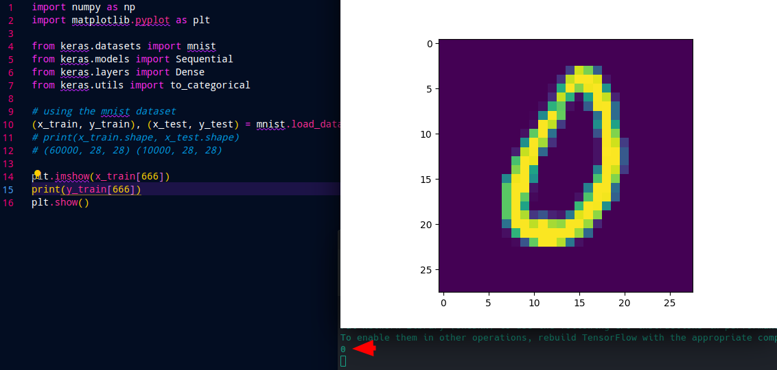
We can print the shape of the dataset to see that we have 60k training images and 10k images for validation - all 28x28 pixel in size. We can also use Matplotlib to display a sample image:
print(x_train.shape, x_test.shape)
# (60000, 28, 28) (10000, 28, 28)

plt.imshow(x_train[666])
plt.show()
To check the assigned label we can run:
print(y_train[666])
# 0
The image shows the number 0 and this is also the assigned label for it:
Data Pre-Processing
The features inside our image are represented with a number range of 0 - 255:
# data pre-processing
## normalize training images
## start by creating a single column 28x28=>784
x_train = x_train.reshape(60000, 784)
x_test = x_test.reshape(10000, 784)

x_train = x_train.astype('float32')
x_test = x_test.astype('float32')

print(x_train[666])
[  ...
   0.   0.   0.   0.   0.   0.   0.   0.   0.   0.   0.   0.   0.   0.
  50. 237. 203.  75.   0.   0.   0.   0.   0.   0.   0.   0.   0.   0.
   0.   0.   0.   0.   0.   0.   0.   0.   0.   0.   0.   0.   0.  37.
 232. 254. 254. 244.  15.   0.   0.   0.   0.   0.   0.   0.   0.   0.
   0.   0.   0.   0.   0.   0.   0.   0.   0.   0.   0.   0.   9. 156.
 254. 209. 250. 254. 131.   0.   0.   0.   0.   0.   0.   0.   0.   0.
   0.   0.   0.   0.   0.   0.   0.   0.   0.   0.   0.   0.  31. 233.
 163.  11. 143. 254. 233.  25.   0.   0.   0.   0.   0.   0.   0.   0.
   0.   0.   0.   0.   0.   0.   0.   0.   0.   0.   0.   9. 164. 192.
  11.   0.  74. 253. 254.  89.   0.   0.   0.   0.   0.   0.   0.   0.
   0.   0.   0.   0.   0.   0.   0.   0.   0.   0.   3. 122. 254. 195.
   0.   0.   0.  95. 254.  89.   0.   0.   0.   0.   0.   0.   0.   0.
   0.   0.   0.   0.   0.   0.   0.   0.   0.   0.   9. 254. 231.  44.
   0.   0.   0. 127. 254. 146.   0.   0.   0.   0.   0.   0.   0.   0.
   0.   0.   0.   0.   0.   0.   0.   0.   0.  11. 192. 254.  95.   0.
   0.   0.   0.  65. 254. 207.   0.   0.   0.   0.   0.   0.   0.   0.
   0.   0.   0.   0.   0.   0.   0.   0.   0. 127. 254. 220.  35.   0.
   0.   0.   0.  12. 254. 237.  45.   0.   0.   0.   0.   0.   0.   0.
   0.   0.   0.   0.   0.   0.   0.   0.  21. 233. 253.  86.   0.   0.
   0.   0.   0.  12. 255. 254.  71.   0.   0.   0.   0.   0.   0.   0.
   0.   0.   0.   0.   0.   0.   0.   0. 181. 254. 249.   0.   0.   0.
   0.   0.   0.  12. 254. 254.  71.   0.   0.   0.   0.   0.   0.   0.
   0.   0.   0.   0.   0.   0.   0.   0. 208. 254. 148.   0.   0.   0.
   0.   0.   0. 113. 254. 237.  45.   0.   0.   0.   0.   0.   0.   0.
   0.   0.   0.   0.   0.   0.   0. 119. 250. 254. 129.   0.   0.   0.
   0.   0.   0. 183. 254. 207.   0.   0.   0.   0.   0.   0.   0.   0.
   0.   0.   0.   0.   0.   0.   0. 190. 254. 254.  13.   0.   0.   0.
   0.   0. 112. 254. 254.  91.   0.   0.   0.   0.   0.   0.   0.   0.
   0.   0.   0.   0.   0.   0.   0. 190. 254. 192.   5.   0.   0.   0.
   0.  12. 185. 254. 251.  78.   0.   0.   0.   0.   0.   0.   0.   0.
   0.   0.   0.   0.   0.   0.   0. 190. 254. 147.   0.   0.   0.   0.
   0. 173. 254. 252. 128.   0.   0.   0.   0.   0.   0.   0.   0.   0.
   0.   0.   0.   0.   0.   0.   0. 190. 254. 225.  40.  66.  25.  16.
 102. 243. 254. 212.   0.   0.   0.   0.   0.   0.   0.   0.   0.   0.
   0.   0.   0.   0.   0.   0.   0.  96. 254. 254. 230. 254. 221. 214.
 254. 254. 217.  28.   0.   0.   0.   0.   0.   0.   0.   0.   0.   0.
   0.   0.   0.   0.   0.   0.   0.  10. 167. 254. 254. 254. 254. 254.
 254. 217.  86.   0.   0.   0.   0.   0.   0.   0.   0.   0.   0.   0.
   0.   0.   0.   0.   0.   0.   0.   0.   6.  67. 194. 254. 254. 227.
 100.  11.   0.   0.   0.   0.   0.   0.   0.   0.   0.   0.   0.   0.
   0.   0.   0.   0.   0.   0.   0.   0.   0.   0.   0.   0.   0.   0.
   ...
   ]
We have to normalize them to range between 0 and 1 by dividing their values by 255:
x_train /=255
x_test /=255
Now we have to represent the labels as vectors - so turning our 0 label into [1. 0. 0. 0. 0. 0. 0. 0. 0. 0.]. And Keras provides us with the right utility to do that - to_categorical():
# vectorize labels for the 10 categories from 0-9
y_train = to_categorical(y_train, 10)
y_test = to_categorical(y_test, 10)
print(y_train[666])
# [1. 0. 0. 0. 0. 0. 0. 0. 0. 0.]
Building the Model
We need to build a sequential model with two dense layers. The first one receives our preprocessed images that have a shape of 28x28=784. In the second layer the input shape is given by the previous layer and does not need to be defined. The output uses a softmax activation - so all label will receive a probability and in the end we will pick the one that has the highest to be our predicted label:
- Activation Functions
- relu function: Rectified linear unit activation function
- sigmoid function: For binary classifications
- softmax function: For multi-label classifications
# building the model
model = Sequential()

model.add(Dense(128, activation='relu', input_shape=(784, )))
model.add(Dense(128, activation='relu'))

model.add(Dense(10, activation='softmax'))

model.compile(optimizer='adam', loss='categorical_crossentropy', metrics=['accuracy'])
model.summary()
The compiled model now looks like:
Model: "sequential"
_________________________________________________________________
 Layer (type)                Output Shape              Param #
=================================================================
 dense (Dense)               (None, 128)               100480

 dense_1 (Dense)             (None, 128)               16512

 dense_2 (Dense)             (None, 10)                1290

=================================================================
Total params: 118,282
Trainable params: 118,282
Non-trainable params: 0
_________________________________________________________________
Training the Model
Now we have our data and a model. Next step is to fit the model to our training data and see if we can start making label predictions based off our validation data. Let's start by running a 10 epochs long training cycle using 128 images per batch:
# fitting the model
model.fit(x_train, y_train, batch_size=128, epochs=10)
469/469 [==============================] - 4s 2ms/step - loss: 0.3179 - accuracy: 0.9097
Epoch 2/10
469/469 [==============================] - 1s 2ms/step - loss: 0.1278 - accuracy: 0.9620
Epoch 3/10
469/469 [==============================] - 1s 2ms/step - loss: 0.0882 - accuracy: 0.9731
Epoch 4/10
469/469 [==============================] - 1s 2ms/step - loss: 0.0646 - accuracy: 0.9803
Epoch 5/10
469/469 [==============================] - 1s 2ms/step - loss: 0.0497 - accuracy: 0.9851
Epoch 6/10
469/469 [==============================] - 1s 2ms/step - loss: 0.0403 - accuracy: 0.9875
Epoch 7/10
469/469 [==============================] - 1s 2ms/step - loss: 0.0323 - accuracy: 0.9902
Epoch 8/10
469/469 [==============================] - 1s 2ms/step - loss: 0.0263 - accuracy: 0.9915
Epoch 9/10
469/469 [==============================] - 1s 2ms/step - loss: 0.0220 - accuracy: 0.9929
Epoch 10/10
469/469 [==============================] - 1s 2ms/step - loss: 0.0197 - accuracy: 0.9936
We can see the accuracy increasing from 0.9097 to 0.9936 and the loss decreasing from 0.3179 to 0.0197. To evaluate the fitted model we can now use our validation dataset and see how accurate it can classify those images:
# validation run
val_loss, val_score = model.evaluate(x_test, y_test)
print(val_loss, val_score)
# 0.07639817893505096 0.9789999723434448
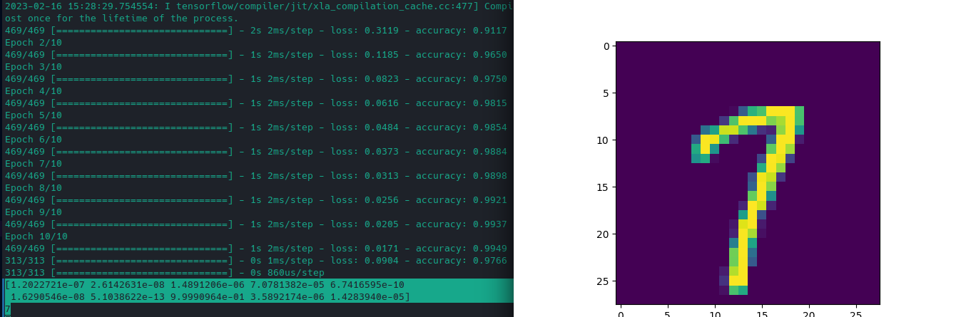
Now it is time to run a prediction with our model:
# run prediction
pred = model.predict(x_test)

## show prediction probabilities
print(pred[666])
## print label with highest probability
pred_max = np.argmax(pred, axis=1)
print(pred_max[666])

## show corresponding image
## reshaping data 784 => 28x28
## to be able to show the image
x = x_test[666].reshape(28, 28)
plt.imshow(x)
plt.show()
The image looks like a 7 and the prediction also assigns 7 by far the highest probability 👍
# prediction probabilities
[8.6091750e-10 4.5242775e-08 6.5181263e-07 1.2005190e-06 1.4038225e-11
 1.9814760e-10 3.8750800e-15 9.9999774e-01 4.4739803e-09 3.6081954e-07]
# predicted label with highest probability
7