• Dimensionality Reduction
  • Dataset
  • RAW Data Analysis
    • 2-Dimensional Plot
    • 3-Dimensional Plot
  • Normalized Data Analysis
    • 2-Dimensional Plot
    • 3-Dimensional Plot
  • Standardized Data Analysis
    • 2-Dimensional Plot
    • 3-Dimensional Plot

Github Repository

t-distributed stochastic neighbor embedding (t-SNE) is a statistical method for visualizing high-dimensional data by giving each datapoint a location in a two or three-dimensional map.

Dimensionality Reduction

Manifold learning is an approach to non-linear dimensionality reduction. Algorithms for this task are based on the idea that the dimensionality of many data sets is only artificially high.

High-dimensional datasets can be very difficult to visualize. While data in two or three dimensions can be plotted to show the inherent structure of the data, equivalent high-dimensional plots are much less intuitive. To aid visualization of the structure of a dataset, the dimension must be reduced in some way.

The simplest way to accomplish this dimensionality reduction is by taking a random projection of the data. Though this allows some degree of visualization of the data structure, the randomness of the choice leaves much to be desired. In a random projection, it is likely that the more interesting structure within the data will be lost.

To address this concern, a number of supervised and unsupervised linear dimensionality reduction frameworks have been designed, such as:

• Principal Component Analysis (PCA)
• Locally Linear Embedding (LLE)
• tStochastic Neighbor Embedding (t-SNE)
• Multidimensional Scaling (MDS)
• Isometric Mapping (ISOMAP)
• Fisher Linear Discriminant Analysis (LDA)

Stochastic Neighbor Embedding with Gaussian and Student-t Distributions: Tutorial and Survey: Stochastic Neighbor Embedding (SNE) is a manifold learning and dimensionality reduction method with a probabilistic approach. In SNE, every point is consider to be the neighbor of all other points with some probability and this probability is tried to be preserved in the embedding space. SNE considers Gaussian distribution for the probability in both the input and embedding spaces. However, t-SNE uses the Student-t and Gaussian distributions in these spaces, respectively. In this tutorial and survey paper, we explain SNE, symmetric SNE, t-SNE (or Cauchy-SNE), and t-SNE with general degrees of freedom. We also cover the out-of-sample extension and acceleration for these methods. Benyamin Ghojogh, Ali Ghodsi, Fakhri Karray, Mark Crowley

Dataset

A multivariate study of variation in two species of rock crab of genus Leptograpsus: A multivariate approach has been used to study morphological variation in the blue and orange-form species of rock crab of the genus Leptograpsus. Objective criteria for the identification of the two species are established, based on the following characters:

• SP: Species (Blue or Orange)
• Sex: Male or Female
• FL: Width of the frontal region of the carapace;
• RW: Width of the posterior region of the carapace (rear width);
• CL: Length of the carapace along the midline;
• CW: Maximum width of the carapace;
• BD: and the depth of the body;

The dataset can be downloaded from Github.

(see introduction in: Principal Component Analysis PCA)

raw_data = pd.read_csv('data/A_multivariate_study_of_variation_in_two_species_of_rock_crab_of_genus_Leptograpsus.csv')

data = raw_data.rename(columns={
    'sp' : 'Species',
    'sex' : 'Sex',
    'index' : 'Index',
    'FL' : 'Frontal Lobe',
    'RW' : 'Rear Width',
    'CL' : 'Carapace Midline',
    'CW' : 'Maximum Width',
    'BD' : 'Body Depth'
})

data['Species'] = data['Species'].map({'B':'Blue', 'O':'Orange'})
data['Sex'] = data['Sex'].map({'M':'Male', 'F':'Female'})

data.head(5)

	Species	Sex	Index	Frontal Lobe	Rear Width	Carapace Midline	Maximum Width	Body Depth
0	Blue	Male	1	8.1	6.7	16.1	19.0	7.0
1	Blue	Male	2	8.8	7.7	18.1	20.8	7.4
2	Blue	Male	3	9.2	7.8	19.0	22.4	7.7
3	Blue	Male	4	9.6	7.9	20.1	23.1	8.2
4	Blue	Male	5	9.8	8.0	20.3	23.0	8.2

# generate a class variable for all 4 classes
data['Class'] = data.Species + data.Sex

print(data['Class'].value_counts())
data.head(1)

• BlueMale: 50
• BlueFemale: 50
• OrangeMale: 50
• OrangeFemale: 50

	species	sex	index	Frontal Lobe	Rear Width	Carapace Midline	Maximum Width	Body Depth	Class
0	Blue	Male	1	8.1	6.7	16.1	19.0	7.0	BlueMale

data_columns = ['Frontal Lobe', 'Rear Width', 'Carapace Midline', 'Maximum Width', 'Body Depth']

RAW Data Analysis

2-Dimensional Plot

# reduce data to 2 dimensions
no_components = 2
no_iter = 2000
perplexity = 10
init = 'random'

data_tsne = TSNE(
    n_components=no_components,
    perplexity=perplexity,
    n_iter=no_iter,
    init=init).fit_transform(data[data_columns])

# add columns to original dataset
data[['TSNE1', 'TSNE2']] = data_tsne

data.tail()

	Species	Sex	Index	Frontal Lobe	Rear Width	Carapace Midline	Maximum Width	Body Depth	Class	TSNE1	TSNE2
195	Orange	Female	46	21.4	18.0	41.2	46.2	18.7	OrangeFemale	39.232815	-1.699857
196	Orange	Female	47	21.7	17.1	41.7	47.2	19.6	OrangeFemale	40.689430	0.257805
197	Orange	Female	48	21.9	17.2	42.6	47.4	19.5	OrangeFemale	41.692440	1.029953
198	Orange	Female	49	22.5	17.2	43.0	48.7	19.8	OrangeFemale	42.851078	2.015537
199	Orange	Female	50	23.1	20.2	46.2	52.5	21.1	OrangeFemale	49.569035	3.964387

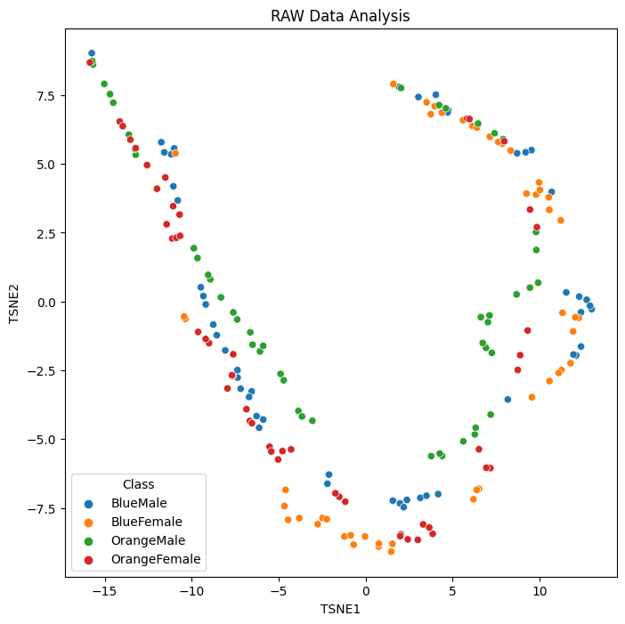
fig = plt.figure(figsize=(8,8))
plt.title('RAW Data Analysis')
sns.scatterplot(x='TSNE1', y='TSNE2', hue='Class', data=data)

3-Dimensional Plot

# reduce data to 3 dimensions
no_components = 3
no_iter = 2000
perplexity = 10
init = 'random'

data_tsne = TSNE(
    n_components=no_components,
    perplexity=perplexity,
    n_iter=no_iter,
    init=init).fit_transform(data[data_columns])

# add columns to original dataset
data[['TSNE1', 'TSNE2', 'TSNE3']] = data_tsne

data.tail()

	Species	Sex	Index	Frontal Lobe	Rear Width	Carapace Midline	Maximum Width	Body Depth	Class	TSNE1	TSNE2	TSNE3
195	Orange	Female	46	21.4	18.0	41.2	46.2	18.7	OrangeFemale	-12.564007	4.956237	-2.111369
196	Orange	Female	47	21.7	17.1	41.7	47.2	19.6	OrangeFemale	-13.217113	5.572454	-2.733016
197	Orange	Female	48	21.9	17.2	42.6	47.4	19.5	OrangeFemale	-13.523155	5.879868	-2.971745
198	Orange	Female	49	22.5	17.2	43.0	48.7	19.8	OrangeFemale	-13.959590	6.371356	-3.287457
199	Orange	Female	50	23.1	20.2	46.2	52.5	21.1	OrangeFemale	-15.850336	8.684433	-3.833084

class_colours = {
    'BlueMale': '#0027c4', #blue
    'BlueFemale': '#f18b0a', #orange
    'OrangeMale': '#0af10a', # green
    'OrangeFemale': '#ff1500', #red
}

colours = data['Class'].apply(lambda x: class_colours[x])

x=data.TSNE1
y=data.TSNE2
z=data.TSNE3

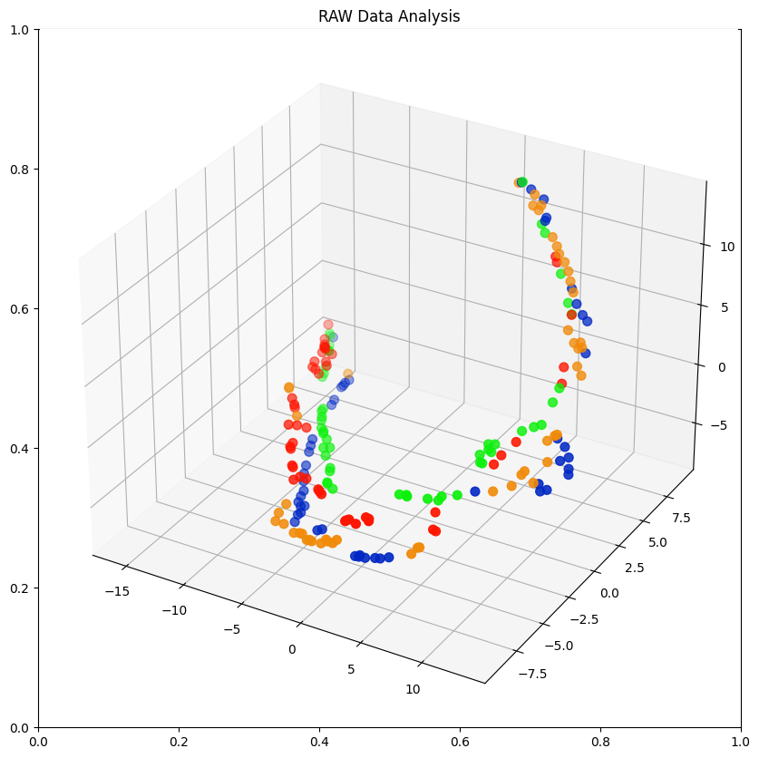
fig = plt.figure(figsize=(10,10))
plt.title('RAW Data Analysis')
ax = fig.add_subplot(projection='3d')

ax.scatter(xs=x, ys=y, zs=z, s=50, c=colours)

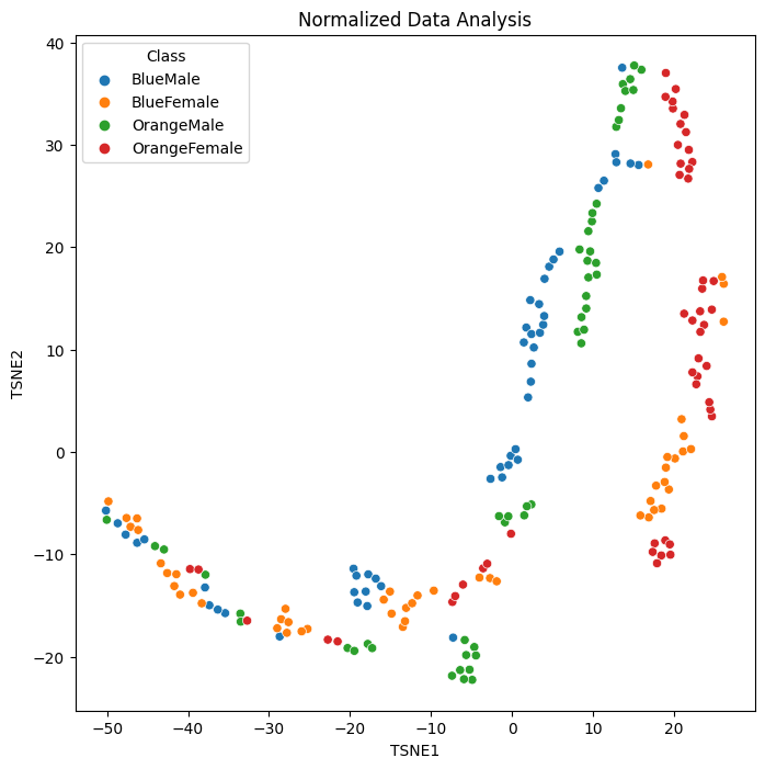
Normalized Data Analysis

2-Dimensional Plot

# normalize the data columns
# values have to be between 0-1
data_norm = data.copy()
data_norm[data_columns] = MinMaxScaler().fit_transform(data[data_columns])

data_norm.describe()

# reduce data to 2 dimensions
no_components = 2
no_iter = 1000
perplexity = 10
init = 'random'

data_tsne = TSNE(
    n_components=no_components,
    perplexity=perplexity,
    n_iter=no_iter,
    init=init).fit_transform(data_norm[data_columns])

# add columns to original dataset
data_norm[['TSNE1', 'TSNE2']] = data_tsne

data_norm.tail()

fig = plt.figure(figsize=(8,8))
plt.title('Normalized Data Analysis')
sns.scatterplot(x='TSNE1', y='TSNE2', hue='Class', data=data_norm)

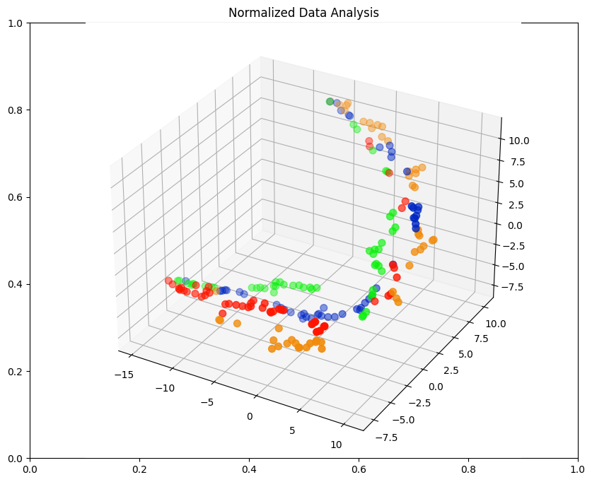
3-Dimensional Plot

# reduce data to 3 dimensions
no_components = 3
no_iter = 1000
perplexity = 10
init = 'random'

data_tsne = TSNE(
    n_components=no_components,
    perplexity=perplexity,
    n_iter=no_iter,
    init=init).fit_transform(data_norm[data_columns])

# add columns to original dataset
data_norm[['TSNE1', 'TSNE2', 'TSNE3']] = data_tsne

data_norm.tail()

class_colours = {
    'BlueMale': '#0027c4', #blue
    'BlueFemale': '#f18b0a', #orange
    'OrangeMale': '#0af10a', # green
    'OrangeFemale': '#ff1500', #red
}

colours = data_norm['Class'].apply(lambda x: class_colours[x])

x=data_norm.TSNE1
y=data_norm.TSNE2
z=data_norm.TSNE3

fig = plt.figure(figsize=(10,8))
plt.title('Normalized Data Analysis')
ax = fig.add_subplot(projection='3d')

ax.scatter(xs=x, ys=y, zs=z, s=50, c=colours)

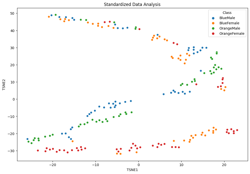
Standardized Data Analysis

2-Dimensional Plot

# standardize date to mean of 0 and std-dev of 1
data_std = data.copy()
data_std[data_columns] = StandardScaler().fit_transform(data[data_columns])

data_std.describe()

# reduce data to 2 dimensions
no_components = 2
no_iter = 1000
perplexity = 10
init = 'random'

data_tsne = TSNE(
    n_components=no_components,
    perplexity=perplexity,
    n_iter=no_iter,
    init=init).fit_transform(data_std[data_columns])

# add columns to original dataset
data_std[['TSNE1', 'TSNE2']] = data_tsne

data_std.tail()

fig = plt.figure(figsize=(12,8))
plt.title('Standardized Data Analysis')
sns.scatterplot(x='TSNE1', y='TSNE2', hue='Class', data=data_std)

3-Dimensional Plot

# reduce data to 3 dimensions
no_components = 3
no_iter = 1000
perplexity = 10
init = 'random'

data_tsne = TSNE(
    n_components=no_components,
    perplexity=perplexity,
    n_iter=no_iter,
    init=init).fit_transform(data_std[data_columns])

# add columns to original dataset
data_std[['TSNE1', 'TSNE2', 'TSNE3']] = data_tsne

data_std.tail()

class_colours = {
    'BlueMale': '#0027c4', #blue
    'BlueFemale': '#f18b0a', #orange
    'OrangeMale': '#0af10a', # green
    'OrangeFemale': '#ff1500', #red
}

colours = data_std['Class'].apply(lambda x: class_colours[x])

x=data_std.TSNE1
y=data_std.TSNE2
z=data_std.TSNE3

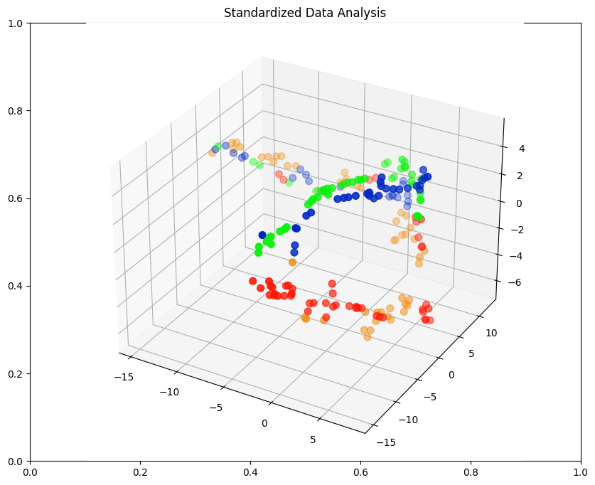
fig = plt.figure(figsize=(10,8))
plt.title('Standardized Data Analysis')
ax = fig.add_subplot(projection='3d')

ax.scatter(xs=x, ys=y, zs=z, s=50, c=colours)