Breast Histopathology Image Segmentation Part 5

- Part 1: Data Inspection and Pre-processing
- Part 2: Weights, Data Augmentations and Generators
- Part 3: Model creation based on a pre-trained and a custom model
- Part 4: Train our model to fit the dataset
- Part 5: Evaluate the performance of your trained model
- Part 6: Running Predictions
Based on Breast Histopathology Images by Paul Mooney.
Invasive Ductal Carcinoma (IDC) is the most common subtype of all breast cancers. To assign an aggressiveness grade to a whole mount sample, pathologists typically focus on the regions which contain the IDC. As a result, one of the common pre-processing steps for automatic aggressiveness grading is to delineate the exact regions of IDC inside of a whole mount slide.Can recurring breast cancer be spotted with AI tech? - BBC News
- Citation: Deep learning for digital pathology image analysis: A comprehensive tutorial with selected use cases
- Dataset: 198,738 IDC(negative) image patches; 78,786 IDC(positive) image patches
Model Evaluation
Classification Report
Generate a Classification Report from your trained model:
- Precision: True Positives / (True Positives + False Positives)
- How certain are you that a positive prediction is actually positive?
- Recall: True Positives / (True Positives + False Negatives)
- How many of the actual positives can be predicted with our model?
- F1 Score: Harmonic mean of precision and recall
- Reaches a maximum when precision and recall are equal
utils/modelEval.py
# Loading the best performing model
# Please specify the model name from the output folder which has the lowest val_loss

# ResNet50
path1 = config.OUTPUT_PATH + '/resnet50_weights-025-0.6333.hdf5'

# Custom
# path1 = config.OUTPUT_PATH + '/custom_weights-009-0.4244.hdf5'

fModel = load_model(path1)

# Predicting on the test data
print("Predicting on the test data")
# if totalTest is odd number add `+1` to predTest
print("totalTrain: " , totalTrain , ", totalVal: " , totalVal , ", totalTest: " , totalTest)
# totalTrain:  199818 , totalVal:  22201 , totalTest:  55505
predTest = fModel.predict(x=testGen, steps=(totalTest // config.BATCH_SIZE)+1)
predTest = np.argmax(predTest, axis=1)

# Printing the Classification Report
print(classification_report(testGen.classes, predTest, target_names=testGen.class_indices.keys()))
Run the script to generate the evaluation report:
ResNet50
              precision    recall  f1-score   support

           0       0.84      0.60      0.70     39775
           1       0.42      0.72      0.53     15730

    accuracy                           0.64     55505
   macro avg       0.63      0.66      0.62     55505
weighted avg       0.72      0.64      0.65     55505
Now this looks pretty terrible :)
Custom
              precision    recall  f1-score   support

           0       0.93      0.84      0.89     39775
           1       0.68      0.84      0.75     15730

    accuracy                           0.84     55505
   macro avg       0.81      0.84      0.82     55505
weighted avg       0.86      0.84      0.85     55505
Already a lot better!
Confusion Matrix
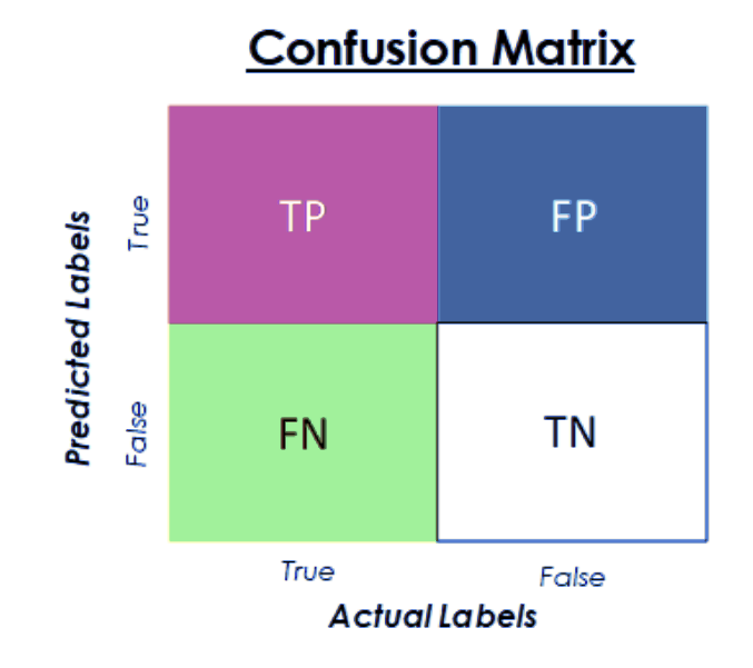
The Confusion Matrix can be used to visualize the performance of an classification model. Since we only have two classes - begin and malignant - the matrix will look like this:
- True Positive: Malignant carcinoma correctly predicted
- False Positive: Malignant carcinoma falsely predicted
- True Negative: Benign carcinoma correctly predicted
- True Negative: Benign carcinoma falsely predicted

utils/modelEval.py
# Computing the confusion matrix and and using the same to derive the
# accuracy, sensitivity, and specificity
cm = confusion_matrix(testGen.classes, predTest)
total = sum(sum(cm))
acc = (cm[0, 0] + cm[1, 1]) / total
sensitivity = cm[0, 0] / (cm[0, 0] + cm[0, 1])
specificity = cm[1, 1] / (cm[1, 0] + cm[1, 1])

# Printing the confusion matrix, accuracy, sensitivity, and specificity
print(cm)
print("acc: {:.4f}".format(acc))
print("sensitivity: {:.4f}".format(sensitivity))
print("specificity: {:.4f}".format(specificity))
ResNet50
[[23954 15821]
 [ 4425 11305]]
acc: 0.6352
sensitivity: 0.6022
specificity: 0.7187
Custom
[[33597  6178]
 [ 2498 13232]]
acc: 0.8437
sensitivity: 0.8447
specificity: 0.8412
AUC-ROC
Area Under the Curve (AUC) of Receiver Operating Characteristic (ROC):
- ROC: Evaluation metric for binary classification problems to separate signal from noise.
- AUC: A measurement of the ability of a classifier to distinguish between classes based on the ROC. A higher value shows a better performance.
## load latest weights
path1 = config.OUTPUT_PATH + '/resnet50_weights.hdf5'

fModel = load_model(path1)

# Predicting on the test data
print("Predicting on the test data")
# if totalTest is odd number add `+1` to predTest
print("totalTrain: " , totalTrain , ", totalVal: " , totalVal , ", totalTest: " , totalTest)
# totalTrain:  199818 , totalVal:  22201 , totalTest:  55505
predTest = fModel.predict(x=testGen, steps=(totalTest // config.BATCH_SIZE)+1)
predTest = np.argmax(predTest, axis=1)

# Calculate roc auc
XGB_roc_value = roc_auc_score(testGen.classes, predTest)
print("XGboost roc_value: {0}" .format(XGB_roc_value))

# Plotting the graph
training_plot(MF, config.EPOCHS, config.PLOT_PATH)
Serializing a Model
When you are satisfied with the training you can save the model so it is ready for transfer:
# Serialize/Writing the model to disk
print("Serializing network...")
fModel.save(config.MODEL_PATH, save_format="h5")
Training Re-run
I changed the following variables:
utils/config.py
BATCH_SIZE = 24
INIT_LR = 1e-3
EPOCHS = 20
For the Custom Model I am still seeing small improvements in the later epochs - looking much better:
Epoch 18/20
8324/8325 [============================>.] - ETA: 0s - loss: 0.4561 - accuracy: 0.8652
Epoch 18: val_loss improved from 0.31292 to 0.31132, saving model to ./output/custom_weights.hdf5
8325/8325 [==============================] - 247s 30ms/step - loss: 0.4561 - accuracy: 0.8652 - val_loss: 0.3113 - val_accuracy: 0.8663
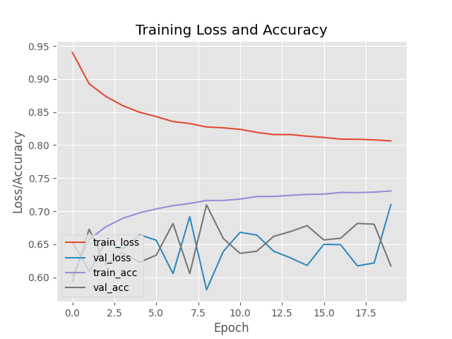
The ResNet50 Model also improves compared to the earlier run. But it still get's stuck around the 10th epoch and even gets much worse after that - given the fluctuation I probably should have let it run a bit longer:
Epoch 9/20
8323/8325 [============================>.] - ETA: 0s - loss: 0.8274 - accuracy: 0.7163
Epoch 9: val_loss improved from 0.60565 to 0.58112, saving model to ./output/resnet50_weights.hdf5
8325/8325 [==============================] - 249s 30ms/step - loss: 0.8274 - accuracy: 0.7163 - val_loss: 0.5811 - val_accuracy: 0.7097

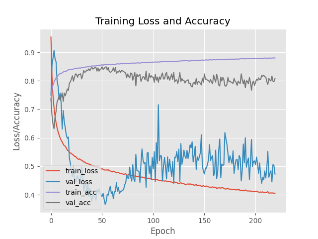
I did another - much longer - run for the Custom Model and I am still seeing improvements up to the 54th epoch. Though the loss function still returns a slightly higher value as before:
Epoch 54/220
8324/8325 [============================>.] - ETA: 0s - loss: 0.4869 - accuracy: 0.8566
Epoch 54: val_loss improved from 0.37685 to 0.36609, saving model to ./output/custom_weights.hdf5
8325/8325 [==============================] - 222s 27ms/step - loss: 0.4869 - accuracy: 0.8566 - val_loss: 0.3661 - val_accuracy: 0.8482
