• Tensorflow Unsupervised Learning
  • Principle of Dimensionality Reduction
    • Build the Autoencoder
    • Train the Autoencoder
    • Visualize the Results
  • Autoencoders for Image Data
    • Building the Autoencoder
    • Run Predictions
  • Autoencoders for Noise Removal
    • Build the Denoise Autoencoder
    • Run Denoiser
  • Food
    • Prepare the Dataset
    • Use an Autoencoder to separate Features

Github Repository

See also:

• Fun, fun, tensors: Tensor Constants, Variables and Attributes, Tensor Indexing, Expanding and Manipulations, Matrix multiplications, Squeeze, One-hot and Numpy
• Tensorflow 2 - Neural Network Regression: Building a Regression Model, Model Evaluation, Model Optimization, Working with a "Real" Dataset, Feature Scaling
• Tensorflow 2 - Neural Network Classification: Non-linear Data and Activation Functions, Model Evaluation and Performance Improvement, Multiclass Classification Problems
• Tensorflow 2 - Convolutional Neural Networks: Binary Image Classification, Multiclass Image Classification
• Tensorflow 2 - Transfer Learning: Feature Extraction, Fine-Tuning, Scaling
• Tensorflow 2 - Unsupervised Learning: Autoencoder Feature Detection, Autoencoder Super-Resolution, Generative Adverserial Networks

Tensorflow Unsupervised Learning

Principle of Dimensionality Reduction

Using Autoencoders to remove "noisy dimensions" in our dataset to be able to extract hidden features.

import matplotlib.pyplot as plt
from mpl_toolkits.mplot3d import Axes3D
import numpy as np
import pandas as pd
import seaborn as sns
from sklearn.datasets import make_blobs
from sklearn.preprocessing import MinMaxScaler
import tensorflow as tf
from tensorflow.keras.datasets import mnist
from tensorflow.keras.layers import Dense, Flatten, Reshape, GaussianNoise
from tensorflow.keras.models import Sequential
from tensorflow.keras.optimizers import SGD, Adam

# global variables
SEED = 42

# create random feature blobs
data = make_blobs(n_samples=300,
                 n_features=2,
                 centers=2,
                 cluster_std=1.0,
                 random_state=SEED)

X, y = data

# create random dataset
np.random.seed(seed=SEED)
z_noise = np.random.normal(size=len(X))
z_noise = pd.Series(z_noise)

# combine data into single dataframe
features = pd.DataFrame(X)
features = pd.concat([features,z_noise], axis=1)
features.columns = ['X1', 'X2', 'Xnoise']

# this generated a dataframe with 3 colums for our data:
print(features.head())

	X1	X2	Xnoise
0	-7.338988	-7.729954	0.496714
1	-7.740041	-7.264665	-0.138264
2	-1.686653	7.793442	0.647689
3	4.422198	3.071947	1.523030
4	-8.917752	-7.888196	-0.234153

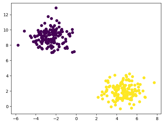
# plotting Y=f(x) shows 2 distinct features
plt.scatter(features['X1'], features['X2'], c=y)

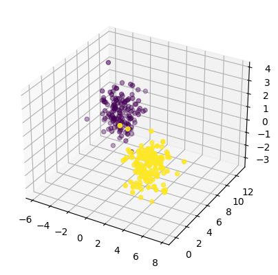
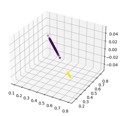
# add a third dimension from the noise data
# this noisy dimension(s) are supposed to
# make it more difficult to see the underlying
# 2 features
fig = plt.figure()
ax = fig.add_subplot(111, projection='3d')
ax.scatter(features['X1'], features['X2'], features['Xnoise'], c=y)

# normalize the dataset
scaler = MinMaxScaler()
scaled_data = scaler.fit_transform(features)

# this generated a dataframe with 3 colums for our data:
print(scaled_data[:5])

array([[0.123409  , 0.0694226 , 0.52692164],
       [0.09881332, 0.09166767, 0.4374124 ],
       [0.4700545 , 0.81158342, 0.54820363],
       [0.84469708, 0.58585258, 0.67159543],
       [0.02658684, 0.06185718, 0.42389547]])

Build the Autoencoder

# build an encoder that reduces dimensionality from 3 => 2
encoder = Sequential([
  Dense(units=2, activation='relu', input_shape=[3])
])

# and an encoder that brings it back up from 2 => 3
decoder = Sequential([
  Dense(units=3, activation='relu', input_shape=[2])
])

# compile both layers into the autoencoder model
autoencoder = Sequential([encoder, decoder])

autoencoder.compile(loss='mse', optimizer=SGD(learning_rate=1.5))

Train the Autoencoder

autoencoder.fit(scaled_data, scaled_data, epochs=5)

# The encoder now reduces the dimensions of our dataset to 2
# when we run predictions from the encoder we will get
# 2-dimensional results that should have stripped the 
# noisy 3rd dimension we added
encoded_2dim = encoder.predict(scaled_data)
# (300, 2) <= (300, 3)
print(encoded_2dim.shape, scaled_data.shape)
encoded_2dim

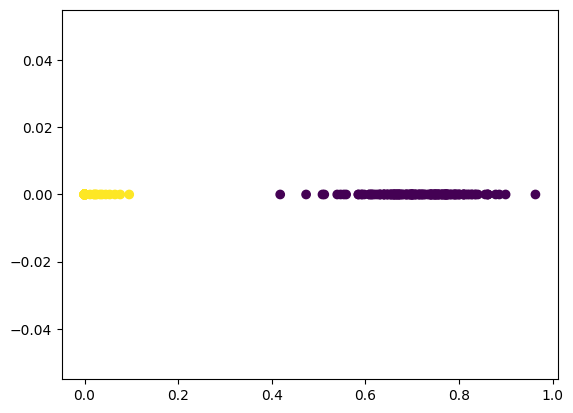
Visualize the Results

plt.scatter(encoded_2dim[:,0], encoded_2dim[:,1], c=y)
# the encoder simplified our dataset and extracted 2 clearly
# defined features that might have been obfuscated by the
# extra dimensions in our dataset

decoded_2to3dim = autoencoder.predict(scaled_data)
print(decoded_2to3dim.shape, scaled_data.shape)
#  (300, 3) <= (300, 2) <= (300, 3)
decoded_2to3dim

fig = plt.figure()
ax = fig.add_subplot(111, projection='3d')
ax.scatter(decoded_2to3dim[:,0], decoded_2to3dim[:,1], decoded_2to3dim[:,2], c=y)

Autoencoders for Image Data

Create a noisy version of the MNIST digits dataset and train an autoencoder to generate de-noised images from this source.

(X_train, y_train), (X_test, y_test) = mnist.load_data()

plt.imshow(X_train[88])

# normalize images
X_train = X_train/255
X_test = X_test/255

Building the Autoencoder

The dataset starts out with 28*28 px images = 784 dimensions. The Encoder should now, several times over several layers, approx. cut this number in half until a minimum of dimensions is reached in a hidden layer.

The following Decoder should then take those reduced feature maps and reconstruct the original image from it. By validating the against the original, not noisy images we should be able to train the Autoencoder to denoise images.

Let's get started by an autoencoder that can read the original image, reduces it to ~3% and then reconstruct the original image from this state:

encoder = Sequential([
    # generate (28, 28) => (784) shape
    Flatten(input_shape=[28, 28], name='input_layer'),
    # cut dimensions in half 
    Dense(units=392, activation='relu', name="reducer50"),
    # cut dimensions in half 
    Dense(units=196, activation='relu', name="reducer25"),
    # cut dimensions in half 
    Dense(units=98, activation='relu', name="reducer12"),
    # cut dimensions in half 
    Dense(units=49, activation='relu', name="reducer6"),
    # cut dimensions in ~ half 
    Dense(units=24, activation='relu', name='hidden_layer')
])

decoder = Sequential([
    Dense(units=49, activation='relu', input_shape=[24], name='expander6'),
    Dense(units=98, activation='relu', name='expander12'),
    Dense(units=98, activation='relu', name='expander25'),
    Dense(units=392, activation='relu', name='expander50'),
    Dense(units=784, activation='sigmoid', name='expander100'),
    Reshape([28, 28], name='output_layer')
])

autoencoder = Sequential([encoder, decoder])

autoencoder.compile(loss='binary_crossentropy',
#                    optimizer=SGD(learning_rate=1.5),
                    optimizer=Adam(learning_rate=1e-3),
                    metrics=['accuracy'])

tf.random.set_seed(SEED)
# fit the autoencoder to training dataset
autoencoder.fit(X_train, X_train, epochs=25,
               validation_data=[X_test, X_test])

# Epoch 25/25
# 6s 3ms/step - loss: 0.0898 - accuracy: 0.3063 - val_loss: 0.0923 - val_accuracy: 0.2968

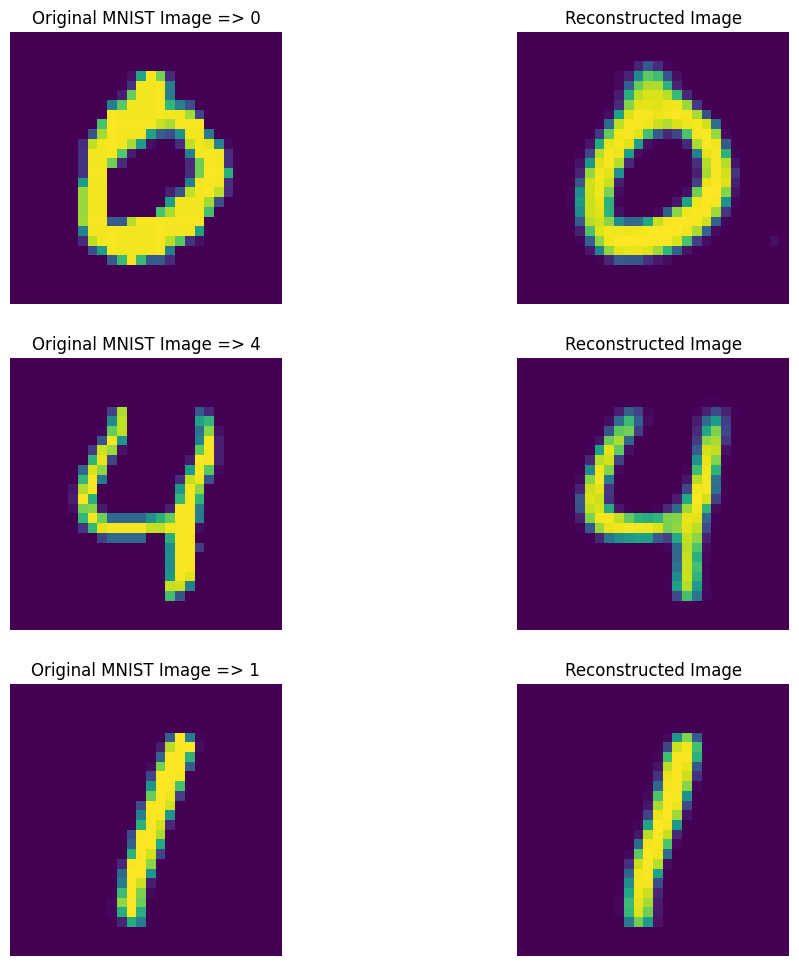
Run Predictions

# get 10 sample predictions from testing dataset
passed_images = autoencoder.predict(X_test[:10])

# select 3 images out of 10 samples
n = [3, 4, 5]

plt.figure(figsize=(12, 12))
# ROW 1
plt.subplot(3, 2, 1)
plt.title(f"Original MNIST Image => {y_test[n[0]]}")
plt.axis(False)
plt.imshow(X_test[n[0]])
plt.subplot(3, 2, 2)
plt.title("Reconstructed Image")
plt.axis(False)
plt.imshow(passed_images[n[0]])
# ROW 2
plt.subplot(3, 2, 3)
plt.title(f"Original MNIST Image => {y_test[n[1]]}")
plt.axis(False)
plt.imshow(X_test[n[1]])
plt.subplot(3, 2, 4)
plt.title("Reconstructed Image")
plt.axis(False)
plt.imshow(passed_images[n[1]])
# ROW 3
plt.subplot(3, 2, 5)
plt.title(f"Original MNIST Image => {y_test[n[2]]}")
plt.axis(False)
plt.imshow(X_test[n[2]])
plt.subplot(3, 2, 6)
plt.title("Reconstructed Image")
plt.axis(False)
plt.imshow(passed_images[n[2]])

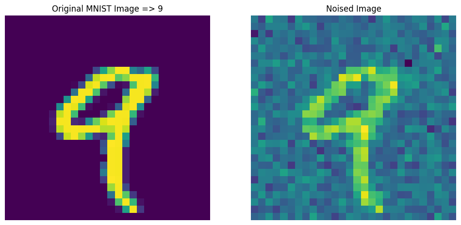
Autoencoders for Noise Removal

# generating noise
sample = GaussianNoise(0.2)
noisy = sample(X_train[:10], training=True)

n = 4

plt.figure(figsize=(12, 12))
# ROW 1
plt.subplot(1, 2, 1)
plt.title(f"Original MNIST Image => {y_train[n]}")
plt.axis(False)
plt.imshow(X_train[n])
plt.subplot(1, 2, 2)
plt.title("Noised Image")
plt.axis(False)
plt.imshow(noisy[n])

Build the Denoise Autoencoder

tf.random.set_seed(SEED)

encoder = Sequential([
    # generate (28, 28) => (784) shape
    Flatten(input_shape=[28, 28], name='input_layer'),
    
    # add noise to source image
    GaussianNoise(0.2),
    
    # cut dimensions in half 
    Dense(units=392, activation='relu', name="reducer50"),
    # cut dimensions in half 
    Dense(units=196, activation='relu', name="reducer25"),
    # cut dimensions in half 
    Dense(units=98, activation='relu', name="reducer12"),
    # cut dimensions in half 
    Dense(units=49, activation='relu', name="reducer6"),
    # cut dimensions in ~ half 
    Dense(units=24, activation='relu', name='hidden_layer')
])

decoder = Sequential([
    Dense(units=49, activation='relu', input_shape=[24], name='expander6'),
    Dense(units=98, activation='relu', name='expander12'),
    Dense(units=98, activation='relu', name='expander25'),
    Dense(units=392, activation='relu', name='expander50'),
    Dense(units=784, activation='sigmoid', name='expander100'),
    Reshape([28, 28], name='output_layer')
])

noise_remover = Sequential([encoder, decoder])

noise_remover.compile(loss='binary_crossentropy',
                     optimizer=Adam(learning_rate=1e-3),
                     metrics=['accuracy'])

noise_remover.fit(X_train, X_train, epochs=25,
               validation_data=[X_test, X_test])

# Epoch 25/25
# 6s 3ms/step - loss: 0.0946 - accuracy: 0.2949 - val_loss: 0.0913 - val_accuracy: 0.2986

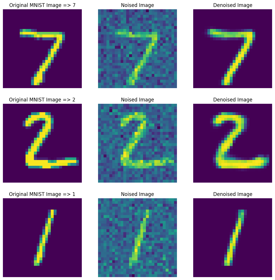
Run Denoiser

noisy_samples = sample(X_test[:3], training=True)

denoised_samples = noise_remover(noisy_samples)

# plot results
plt.figure(figsize=(12, 12))
# ROW 1
plt.subplot(3, 3, 1)
plt.title(f"Original MNIST Image => {y_test[0]}")
plt.axis(False)
plt.imshow(X_test[0])
plt.subplot(3, 3, 2)
plt.title("Noised Image")
plt.axis(False)
plt.imshow(noisy_samples[0])
plt.subplot(3, 3, 3)
plt.title("Denoised Image")
plt.axis(False)
plt.imshow(denoised_samples[0])
# ROW 2
plt.subplot(3, 3, 4)
plt.title(f"Original MNIST Image => {y_test[1]}")
plt.axis(False)
plt.imshow(X_test[1])
plt.subplot(3, 3, 5)
plt.title("Noised Image")
plt.axis(False)
plt.imshow(noisy_samples[1])
plt.subplot(3, 3, 6)
plt.title("Denoised Image")
plt.axis(False)
plt.imshow(denoised_samples[1])
# ROW 3
plt.subplot(3, 3, 7)
plt.title(f"Original MNIST Image => {y_test[2]}")
plt.axis(False)
plt.imshow(X_test[2])
plt.subplot(3, 3, 8)
plt.title("Noised Image")
plt.axis(False)
plt.imshow(noisy_samples[2])
plt.subplot(3, 3, 9)
plt.title("Denoised Image")
plt.axis(False)
plt.imshow(denoised_samples[2])

Food

Variations in preference for different food types in the UK

wget https://github.com/emtrujillo-lab/bggn213/blob/3fdf3e1f373545a420de9fb45a2a8e68ee5478fa/Class09/Class9/UK_foods.csv

Prepare the Dataset

df = pd.read_csv('./UK_foods.csv', index_col='Unnamed: 0')
df

	England	Wales	Scotland	N.Ireland
Cheese	105	103	103	66
Carcass_meat	245	227	242	267
Other_meat	685	803	750	586
Fish	147	160	122	93
Fats_and_oils	193	235	184	209
Sugars	156	175	147	139
Fresh_potatoes	720	874	566	1033
Fresh_Veg	253	265	171	143
Other_Veg	488	570	418	355
Processed_potatoes	198	203	220	187
Processed_Veg	360	365	337	334
Fresh_fruit	1102	1137	957	674
Cereals	1472	1582	1462	1494
Beverages	57	73	53	47
Soft_drinks	1374	1256	1572	1506
Alcoholic_drinks	375	475	458	135
Confectionery	54	64	62	41

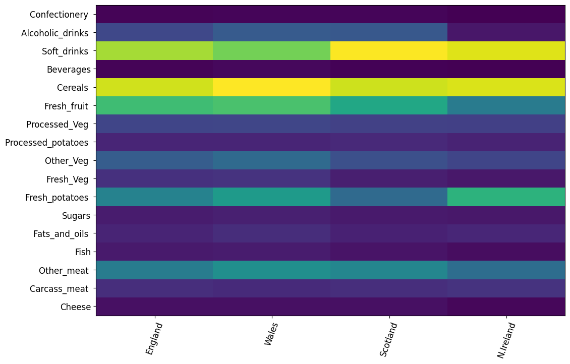
# create a heatmap with pandas
plt.figure(figsize=(12, 8))
plt.pcolor(df)
plt.yticks(np.arange(0.5, len(df.index), 1), df.index)
plt.xticks(np.arange(0.5, len(df.columns), 1), df.columns)
plt.xticks(rotation=70, fontsize=12)
plt.yticks(fontsize=12)
plt.show()

df_t = df.transpose()
df_t

	Cheese	Carcass_meat	Other_meat	Fish	Fats_and_oils	Sugars	Fresh_potatoes	Fresh_Veg	Other_Veg	Processed_potatoes	Processed_Veg	Fresh_fruit	Cereals	Beverages	Soft_drinks	Alcoholic_drinks	Confectionery
England	105	245	685	147	193	156	720	253	488	198	360	1102	1472	57	1374	375	54
Wales	103	227	803	160	235	175	874	265	570	203	365	1137	1582	73	1256	475	64
Scotland	103	242	750	122	184	147	566	171	418	220	337	957	1462	53	1572	458	62
N.Ireland	66	267	586	93	209	139	1033	143	355	187	334	674	1494	47	1506	135	41

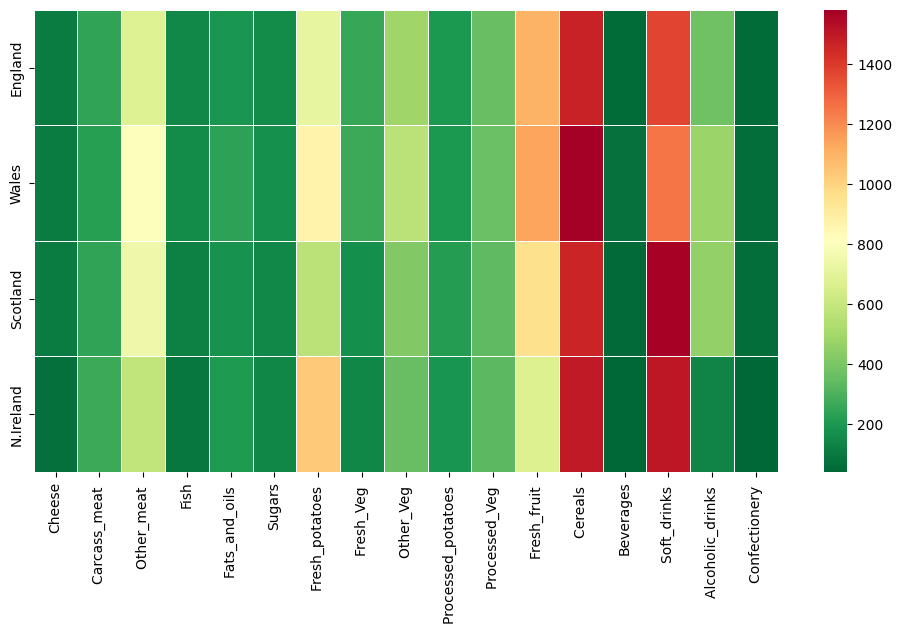
# create a heatmap with seaborn
plt.figure(figsize=(12, 6))
sns.heatmap(df_t, cmap='RdYlGn_r', linewidths=0.5, annot=False)

Use an Autoencoder to separate Features

# build the autoencoder
encoder = Sequential([
    Dense(units=8, activation='relu', input_shape=[17]),
    Dense(units=4, activation='relu'),
    Dense(units=2, activation='relu')
])

decoder = Sequential([
    Dense(units=4, activation='relu', input_shape=[2]),
    Dense(units=8, activation='relu'),
    Dense(units=17, activation='relu')
])

autoencoder= Sequential([encoder, decoder])

autoencoder.compile(loss='mse', optimizer=Adam(learning_rate=1e-3))

# normalize input data
scaler = MinMaxScaler()

scaled_df = scaler.fit_transform(df_t.values)
scaled_df.shape
# (4, 17)

autoencoder.fit(scaled_df, scaled_df, epochs=25)
# Epoch 25/25
# 1/1 [==============================] - 0s 5ms/step - loss: 0.2891

# get reduced dimensionality output from encoder
encoded_2dim = encoder.predict(scaled_df)
encoded_2dim

# array([[0.        , 1.8262266 ],
#        [0.        , 3.4182868 ],
#        [0.        , 1.7019984 ],
#        [0.20801371, 0.52220476]], dtype=float32)

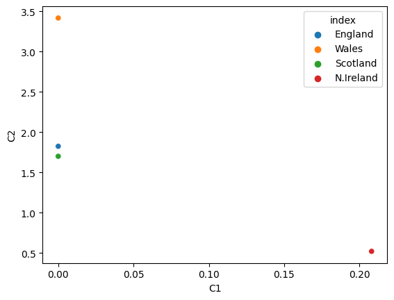
results = pd.DataFrame(data=encoded_2dim,
                      index=df_t.index,
                      columns=['C1', 'C2'])

results.reset_index()

	index	C1	C2
0	England	0.000000	1.826227
1	Wales	0.000000	3.418287
2	Scotland	0.000000	1.701998
3	N.Ireland	0.208014	0.522205

sns.scatterplot(x='C1', y='C2', data=results.reset_index(), hue='index')

# England and Scotland are very close to each other
# while Wales and N.Ireland