• Dimensionality Reduction
  • Dataset
  • 2-Dimensional Plot
  • 3-Dimensional Plot

Github Repository

Fisher's linear discriminant, a method used in statistics and other fields, to find a linear combination of features that characterizes or separates two or more classes of objects or events. The resulting combination may be used as a linear classifier, or, more commonly, for dimensionality reduction before later classification.

Fisher and Kernel Fisher Discriminant Analysis: Tutorial: This is a detailed tutorial paper which explains the Fisher discriminant Analysis (FDA) and kernel FDA. We start with projection and reconstruction. Then, one- and multi-dimensional FDA subspaces are covered. Scatters in two- and then multi-classes are explained in FDA. Then, we discuss on the rank of the scatters and the dimensionality of the subspace. A real-life example is also provided for interpreting FDA. Then, possible singularity of the scatter is discussed to introduce robust FDA. PCA and FDA directions are also compared. We also prove that FDA and linear discriminant analysis are equivalent. Fisher forest is also introduced as an ensemble of fisher subspaces useful for handling data with different features and dimensionality. Afterwards, kernel FDA is explained for both one- and multi-dimensional subspaces with both two- and multi-classes. Finally, some simulations are performed on AT&T face dataset to illustrate FDA and compare it with PCA. Benyamin Ghojogh, Fakhri Karray, Mark Crowley

Dimensionality Reduction

Manifold learning is an approach to non-linear dimensionality reduction. Algorithms for this task are based on the idea that the dimensionality of many data sets is only artificially high.

High-dimensional datasets can be very difficult to visualize. While data in two or three dimensions can be plotted to show the inherent structure of the data, equivalent high-dimensional plots are much less intuitive. To aid visualization of the structure of a dataset, the dimension must be reduced in some way.

The simplest way to accomplish this dimensionality reduction is by taking a random projection of the data. Though this allows some degree of visualization of the data structure, the randomness of the choice leaves much to be desired. In a random projection, it is likely that the more interesting structure within the data will be lost.

To address this concern, a number of supervised and unsupervised linear dimensionality reduction frameworks have been designed, such as:

• Principal Component Analysis (PCA)
• Locally Linear Embedding (LLE)
• tStochastic Neighbor Embedding (t-SNE)
• Multidimensional Scaling (MDS)
• Isometric Mapping (ISOMAP)
• Fisher Linear Discriminant Analysis (LDA)

Dataset

A multivariate study of variation in two species of rock crab of genus Leptograpsus: A multivariate approach has been used to study morphological variation in the blue and orange-form species of rock crab of the genus Leptograpsus. Objective criteria for the identification of the two species are established, based on the following characters:

• SP: Species (Blue or Orange)
• Sex: Male or Female
• FL: Width of the frontal region of the carapace;
• RW: Width of the posterior region of the carapace (rear width);
• CL: Length of the carapace along the midline;
• CW: Maximum width of the carapace;
• BD: and the depth of the body;

The dataset can be downloaded from Github.

(see introduction in: Principal Component Analysis PCA)

raw_data = pd.read_csv('data/A_multivariate_study_of_variation_in_two_species_of_rock_crab_of_genus_Leptograpsus.csv')

data = raw_data.rename(columns={
    'sp': 'Species',
    'sex': 'Sex',
    'index': 'Index',
    'FL': 'Frontal Lobe',
    'RW': 'Rear Width',
    'CL': 'Carapace Midline',
    'CW': 'Maximum Width',
    'BD': 'Body Depth'})

data['Species'] = data['Species'].map({'B':'Blue', 'O':'Orange'})
data['Sex'] = data['Sex'].map({'M':'Male', 'F':'Female'})
data['Class'] = data.Species + data.Sex

data_columns = ['Frontal Lobe',
                'Rear Width',
                'Carapace Midline',
                'Maximum Width',
                'Body Depth']

# generate a class variable for all 4 classes
data['Class'] = data.Species + data.Sex

print(data['Class'].value_counts())
data.head(5)

• BlueMale: 50
• BlueFemale: 50
• OrangeMale: 50
• OrangeFemale: 50

	Species	Sex	Index	Frontal Lobe	Rear Width	Carapace Midline	Maximum Width	Body Depth	Class
0	Blue	Male	1	8.1	6.7	16.1	19.0	7.0	BlueMale
1	Blue	Male	2	8.8	7.7	18.1	20.8	7.4	BlueMale
2	Blue	Male	3	9.2	7.8	19.0	22.4	7.7	BlueMale
3	Blue	Male	4	9.6	7.9	20.1	23.1	8.2	BlueMale
4	Blue	Male	5	9.8	8.0	20.3	23.0	8.2	BlueMale

# normalize data columns
data_norm = data.copy()
data_norm[data_columns] = MinMaxScaler().fit_transform(data[data_columns])

data_norm.describe()

	Index	Frontal Lobe	Rear Width	Carapace Midline	Maximum Width	Body Depth
count	200.000000	200.000000	200.000000	200.000000	200.000000	200.000000
mean	25.500000	0.527233	0.455365	0.529043	0.515053	0.511645
std	14.467083	0.219832	0.187835	0.216382	0.209919	0.220953
min	1.000000	0.000000	0.000000	0.000000	0.000000	0.000000
25%	13.000000	0.358491	0.328467	0.382219	0.384000	0.341935
50%	25.500000	0.525157	0.459854	0.528875	0.525333	0.503226
75%	38.000000	0.682390	0.569343	0.684650	0.664000	0.677419
max	50.000000	1.000000	1.000000	1.000000	1.000000	1.000000

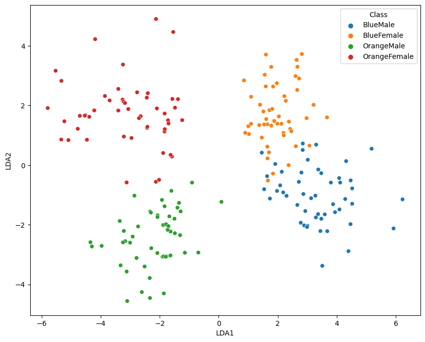
2-Dimensional Plot

no_components = 2

lda = LinearDiscriminantAnalysis(n_components = no_components)
data_lda = lda.fit_transform(data_norm[data_columns].values , y=data_norm['Class'])

data_norm[['LDA1', 'LDA2']] = data_lda

data_norm.head(1)

	Species	Sex	Index	Frontal Lobe	Rear Width	Carapace Midline	Maximum Width	Body Depth	Class	LDA1	LDA2
0	Blue	Male	1	0.056604	0.014599	0.042553	0.050667	0.058065	BlueMale	1.538869	-0.808137

fig = plt.figure(figsize=(10, 8))
sns.scatterplot(x='LDA1', y='LDA2', hue='Class', data=data_norm)

3-Dimensional Plot

no_components = 3

lda = LinearDiscriminantAnalysis(n_components = no_components)
data_lda = lda.fit_transform(data_norm[data_columns].values , y=data_norm['Class'])

data_norm[['LDA1', 'LDA2', 'LDA3']] = data_lda

data_norm.head(1)

	Species	Sex	Index	Frontal Lobe	Rear Width	Carapace Midline	Maximum Width	Body Depth	Class	LDA1	LDA2	LDA3
0	Blue	Male	1	0.056604	0.014599	0.042553	0.050667	0.058065	BlueMale	1.538869	-0.808137	1.18642

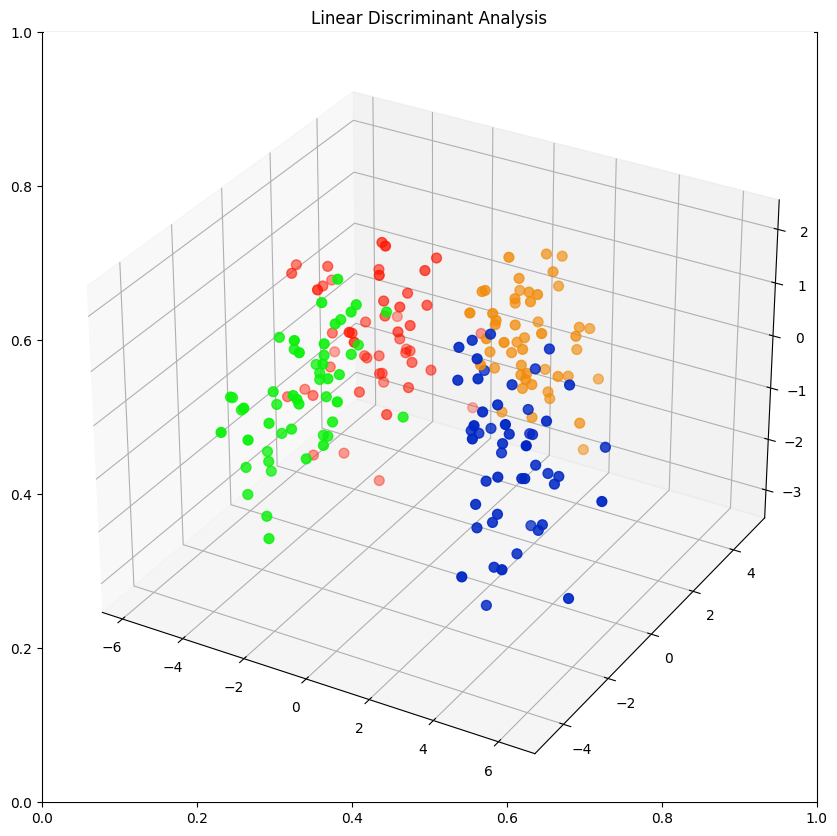
class_colours = {
    'BlueMale': '#0027c4', #blue
    'BlueFemale': '#f18b0a', #orange
    'OrangeMale': '#0af10a', # green
    'OrangeFemale': '#ff1500', #red
}

colours = data_norm['Class'].apply(lambda x: class_colours[x])

x=data_norm.LDA1
y=data_norm.LDA2
z=data_norm.LDA3

fig = plt.figure(figsize=(10,10))
plt.title('Linear Discriminant Analysis')
ax = fig.add_subplot(projection='3d')

ax.scatter(xs=x, ys=y, zs=z, s=50, c=colours)