See also:
- Fun, fun, tensors: Tensor Constants, Variables and Attributes, Tensor Indexing, Expanding and Manipulations, Matrix multiplications, Squeeze, One-hot and Numpy
- Tensorflow 2 - Neural Network Regression: Building a Regression Model, Model Evaluation, Model Optimization, Working with a "Real" Dataset, Feature Scaling
- Tensorflow 2 - Neural Network Classification: Non-linear Data and Activation Functions, Model Evaluation and Performance Improvement, Multiclass Classification Problems
- Tensorflow 2 - Convolutional Neural Networks: Binary Image Classification, Multiclass Image Classification
- Tensorflow 2 - Transfer Learning: Feature Extraction, Fine-Tuning, Scaling
- Tensorflow 2 - Unsupervised Learning: Autoencoder Feature Detection, Autoencoder Super-Resolution, Generative Adverserial Networks
Tensorflow Neural Network Classification
Evaluating a models performance and tweaking the training.
Training & Testing Datasplit
In the example earlier I used a single dataset to both train and test the model. Let's split this dataset so that we have a fresh testing dataset for the model.
# training and testing data split using scikit-learn
X_train, X_test, y_train, y_test = train_test_split(
    X, y, test_size=0.20, random_state=42)

# check shape
X_train.shape, X_test.shape, y_train.shape, y_test.shape
# ((800, 2), (200, 2), (800,), (200,))
# rebuild the best model from above
# train on training set and eval on testing
tf.random.set_seed(42)

model_circles_lr10e_3 = tf.keras.Sequential([
    tf.keras.layers.Dense(4, activation="relu", name="input_layer"),
    tf.keras.layers.Dense(4, activation="relu", name="dense_layer"),
    tf.keras.layers.Dense(1, activation="sigmoid", name="output_layer")
])

model_circles_lr10e_3.compile(loss="binary_crossentropy",
                       optimizer=tf.keras.optimizers.Adam(learning_rate=0.001),
                       metrics=["accuracy"])

history_lr10e_3 = model_circles_lr10e_3.fit(X_train, y_train,
                    validation_data=(X_test, y_test),
                    epochs=2000)

# Epoch 2000/2000
# 25/25 [==============================] - 0s 4ms/step - loss: 2.2199e-04 - accuracy: 1.0000 - val_loss: 0.0131 - val_accuracy: 0.9950
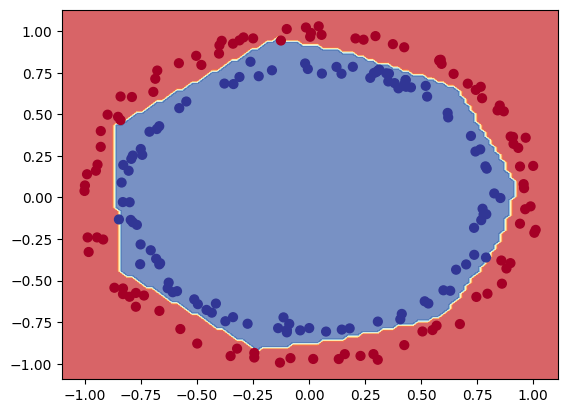
decision_boundray(model=model_circles_lr10e_3, X=X_test, y=y_test)
Learning Rate
In the example above it took 256 cycles to get to an val_accuracy: 0.9000:
25/25 [==============================] - 0s 3ms/step - loss: 0.2355 - accuracy: 0.9100 - val_loss: 0.2647 - val_accuracy: 0.8950
Epoch 255/2000
25/25 [==============================] - 0s 3ms/step - loss: 0.2338 - accuracy: 0.9137 - val_loss: 0.2636 - val_accuracy: 0.8900
Epoch 256/2000
25/25 [==============================] - 0s 3ms/step - loss: 0.2312 - accuracy: 0.9162 - val_loss: 0.2595 - val_accuracy: 0.9000
Epoch 257/2000
25/25 [==============================] - 0s 3ms/step - loss: 0.2255 - accuracy: 0.9162 - val_loss: 0.2390 - val_accuracy: 0.9000
Epoch 258/2000
25/25 [==============================] - 0s 3ms/step - loss: 0.2030 - accuracy: 0.9438 - val_loss: 0.2118 - val_accuracy: 0.9600
By increasing the learning rate we allow Tensorflow to make bigger changes to the model weights after each epoch. This should increase the initial speed with which the model is moving towards the optimum:
tf.random.set_seed(42)

model_circles_lr10e_2 = tf.keras.Sequential([
    tf.keras.layers.Dense(4, activation="relu", name="input_layer"),
    tf.keras.layers.Dense(4, activation="relu", name="dense_layer"),
    tf.keras.layers.Dense(1, activation="sigmoid", name="output_layer")
])

model_circles_lr10e_2.compile(loss="binary_crossentropy",
                       optimizer=tf.keras.optimizers.Adam(learning_rate=0.01),
                       metrics=["accuracy"])

history_lr10e_2 = model_circles_lr10e_2.fit(X_train, y_train,
                    validation_data=(X_test, y_test),
                    epochs=2000)

# Epoch 2000/2000
# 25/25 [==============================] - 0s 3ms/step - loss: 4.2108e-04 - accuracy: 1.0000 - val_loss: 0.0158 - val_accuracy: 0.9900
With the increases learning rate we alread reach 90% after 25 epochs:
25/25 [==============================] - 0s 3ms/step - loss: 0.4151 - accuracy: 0.8475 - val_loss: 0.4481 - val_accuracy: 0.8050
Epoch 14/2000
25/25 [==============================] - 0s 3ms/step - loss: 0.3880 - accuracy: 0.8625 - val_loss: 0.4032 - val_accuracy: 0.8700
Epoch 15/2000
25/25 [==============================] - 0s 4ms/step - loss: 0.3304 - accuracy: 0.9025 - val_loss: 0.2930 - val_accuracy: 0.9550
Epoch 16/2000
25/25 [==============================] - 0s 3ms/step - loss: 0.2191 - accuracy: 0.9937 - val_loss: 0.2185 - val_accuracy: 1.0000
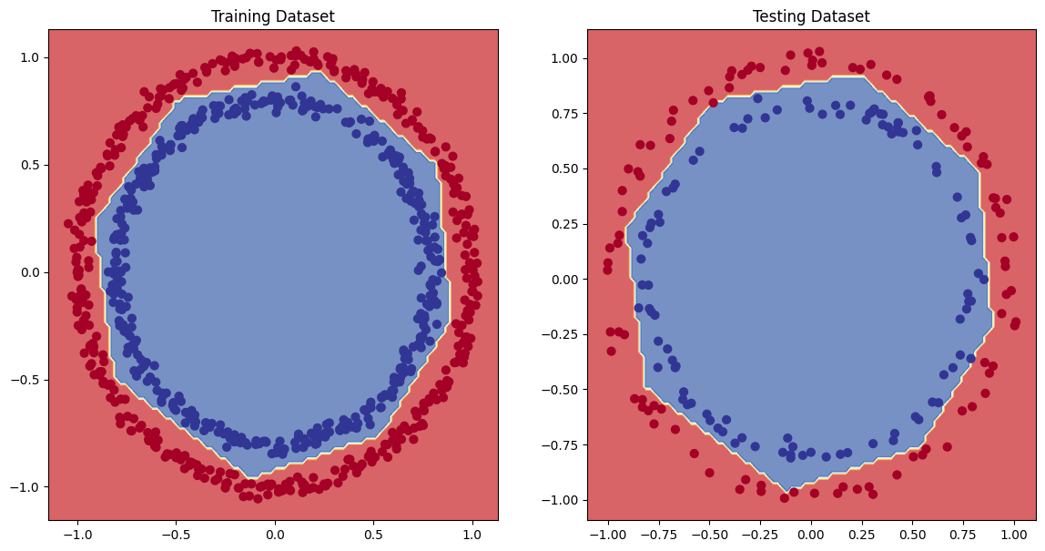
plt.figure(figsize=(14, 7))
plt.subplot(1, 2, 1)
plt.title("Training Dataset")
decision_boundray(model=model_circles_lr10e_2, X=X_train, y=y_train)
plt.subplot(1, 2, 2)
plt.title("Testing Dataset")
decision_boundray(model=model_circles_lr10e_2, X=X_test, y=y_test)
plt.show()
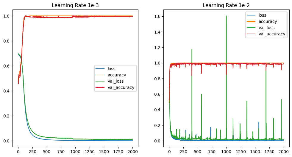
Finding the ideal learning rate
Comparing the learning progress of the previous two identical experiments - with a difference in learning rate 1e-3 vs 1e-2
fig, axes = plt.subplots(nrows=1, ncols=2, figsize=(12, 6))
pd.DataFrame(history_lr10e_3.history).plot(ax=axes[0], title="Learning Rate 1e-3")
pd.DataFrame(history_lr10e_2.history).plot(ax=axes[1], title="Learning Rate 1e-2")
# with a larger learning rate the loss/accuracy improves much quicker
# but a larger learning rate also means that we get some overshots / fluctuations in performance
Dynamically adjust the Learning Rate
We can use the Keras LearningRateScheduler() in a Callback to update the learning rate of the used optimizer according to the schedule function with each new epoch.
# create a new model based on model_circles_lr10e_3
tf.random.set_seed(7)
model_circles_lr_callback = tf.keras.Sequential([
tf.keras.layers.Dense(4, activation="relu", name="input_layer"),
tf.keras.layers.Dense(4, activation="relu", name="dense_layer"),
tf.keras.layers.Dense(1, activation="sigmoid", name="output_layer")
])
model_circles_lr_callback.compile(loss="binary_crossentropy",
optimizer=tf.keras.optimizers.Adam(learning_rate=0.001),
metrics=["accuracy"])
# introduce learning scheduler callback to increase the learning rate
# with every epoch by `0.0001 times 10e(epoch/100)`
learning_rate_callback = tf.keras.callbacks.LearningRateScheduler(lambda epoch: 1e-4 * 10**(epoch/100))
history_lr_callback = model_circles_lr_callback.fit(X_train, y_train,
validation_data=(X_test, y_test), epochs=500,
callbacks=[learning_rate_callback], verbose=1)
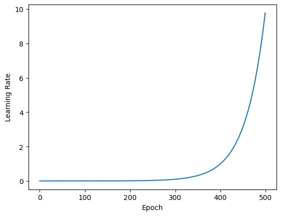
# the learning rate, initially, increases sensibly. But later explodes leading to a terrible performance:
# Epoch 500/500
# 25/25 [==============================] - 0s 3ms/step - loss: 0.7646 - accuracy: 0.5025 - val_loss: 0.6961 - val_accuracy: 0.5000 - lr: 9.7724
# plot the learning rate progression
lr = 1e-4 * (10 ** (tf.range(500)/100))
plt.plot(tf.range(500), lr)
plt.ylabel("Learning Rate")
plt.xlabel("Epoch")
plt.show()
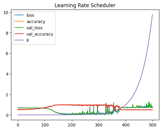
# the adaptive learning rate stays reasonable up until the 300th epoch
pd.DataFrame(history_lr_callback.history).plot(title="Learning Rate Scheduler")
# and the learning rate abve the 200th epoch leads to more and more fluctuations in loss and accuracy.
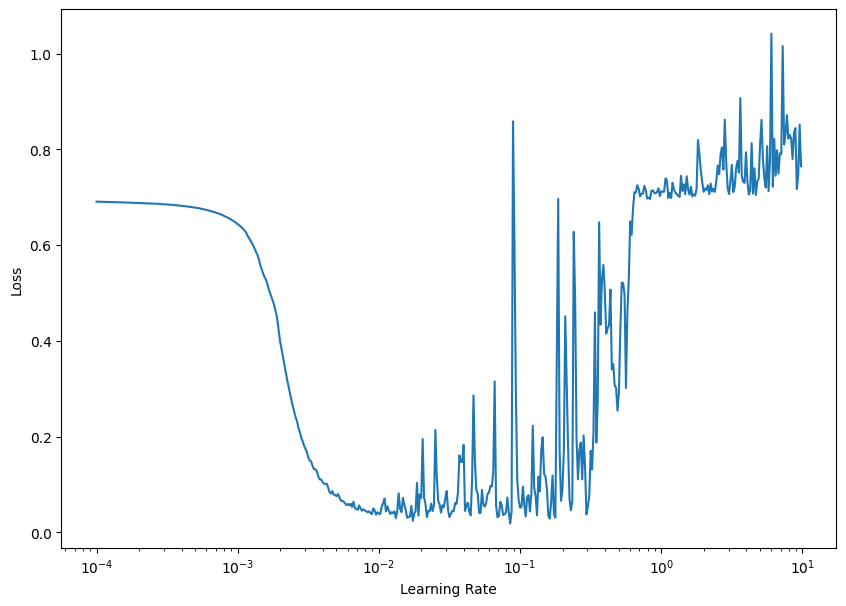
# the "ideal learning rate" is usally 10 times smaller than the value at the bottom of the loss curve (`loss = f(lr)`)
plt.figure(figsize=(10, 7))
plt.xlabel("Learning Rate")
plt.ylabel("Loss")
plt.semilogx(lr, history_lr_callback.history["loss"])
plt.show()
# for the plot below this would be around `3*10e-3` and `4*10e-3`
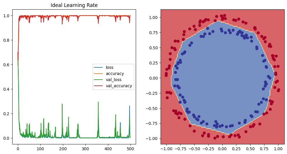
# re-run the model with the ideal learning rate
tf.random.set_seed(42)

model_circles_ideal_lr = tf.keras.Sequential([
    tf.keras.layers.Dense(4, activation="relu", name="input_layer"),
    tf.keras.layers.Dense(4, activation="relu", name="dense_layer"),
    tf.keras.layers.Dense(1, activation="sigmoid", name="output_layer")
])

model_circles_ideal_lr.compile(loss="binary_crossentropy",
                                 optimizer=tf.keras.optimizers.Adam(learning_rate=4*10e-3),
                                 metrics=["accuracy"])

history_ideal_lr = model_circles_ideal_lr.fit(X_train, y_train,
                                      validation_data=(X_test, y_test),
                                      epochs=500, verbose=1)

# Epoch 500/500
# 25/25 [==============================] - 0s 3ms/step - loss: 0.0038 - accuracy: 1.0000 - val_loss: 0.0100 - val_accuracy: 1.0000
fig, axes = plt.subplots(nrows=1, ncols=2, figsize=(12, 6))
pd.DataFrame(history_ideal_lr.history).plot(ax=axes[0], title="Ideal Learning Rate")
decision_boundray(model=model_circles_ideal_lr, X=X_test, y=y_test)
Confusion Matrix
So far I used Accuracy as metric to evaluate the performance of a trained model. But accuracy can fall short of representing a dataset with imbalanced classes. If a class only makes up 1% of a dataset even if our model fails 100% of the time to predict the class we still end up with a high accuracy overall:
- Accuracy = (tp + tn) / (tp + tn + fp + fn)
tf.keras.metrics.Accuracy(),sklearn.metrics.accuracy_score()
A metric that allows us to indicate the amount of false positive predictions is Precision:
- Precision = tp / (tp + fp)
tf.keras.metrics.Precision(),sklearn.metrics.precision_score()
A metric to evaluate the amount of false negative predictions is Recall:
- Recall = tp / (tp + fn)
tf.keras.metrics.Recall(),sklearn.metrics.recall_score()
Depending on our problem we can use precision or recall instead of accuracy as the training performance metric. A metric that combines both recall and precision is the F1 Score in SciKit_Learn:
- F1-score = 2 * (precision * recall)/(precision + recall)
sklearn.metrics.f1_score()
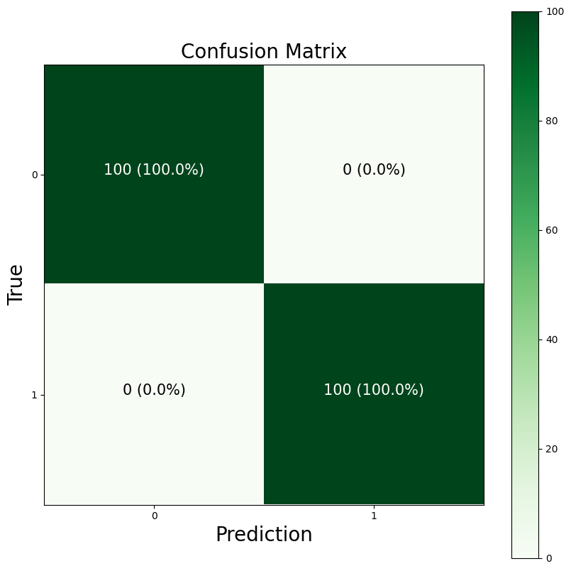
A good visual representation of a models performance is the Confusion Matrix that compares predictions to the true value sklearn.metrics.confusion_matrix().
# check loss and accuracy of the previous model
loss, accuracy = model_circles_ideal_lr.evaluate(X_test, y_test)
print(f"INFO :: Model loss - {loss:.5f}")
print(f"INFO :: Model accuracy - {(accuracy*100):.2f}%")
# 7/7 [==============================] - 0s 2ms/step - loss: 0.0100 - accuracy: 1.0000
# INFO :: Model loss - 0.01005
# INFO :: Model accuracy - 100.00%
# confusion matrix
## get label predictions using the trained model
y_pred = model_circles_ideal_lr.predict(X_test)
# y_pred, y_test
# the predictions we get are floats while the true values are binary `1` or `0`
# round the prediction to be able to compare them:
y_pred_rnd = tf.round(y_pred)
confusion_matrix(y_pred_rnd, y_test)
# array([[100,   0],
#        [  0, 100]])
# plot confusion matrix
import itertools

def plot_confusion_matrix(y_pred=y_pred_rnd, y_test=y_test):
        figsize = (10, 10)

        # create the confusion matrix
        cm = confusion_matrix(y_pred_rnd, y_test)

        # normalize
        cm_norm = cm.astype("float") / cm.sum(axis=1)[:, np.newaxis]
        # cm_norm
        # array([[1., 0.],
        #        [0., 1.]])

        number_of_classes = cm.shape[0]
        # 2

        # plot matrix
        fig, ax = plt.subplots(figsize=figsize)
        cax = ax.matshow(cm, cmap=plt.cm.Greens)
        fig.colorbar(cax)

        # create classes
        classes = False

        if classes:
            labels = classes
        else:
            labels = np.arange(cm.shape[0])

        # axes lables
        ax.set(title="Confusion Matrix",
              xlabel="Prediction",
              ylabel="True",
              xticks=np.arange(number_of_classes),
              yticks=np.arange(number_of_classes),
              xticklabels=labels,
              yticklabels=labels)

        ax.xaxis.set_label_position("bottom")
        ax.title.set_size(20)
        ax.xaxis.label.set_size(20)
        ax.yaxis.label.set_size(20)
        ax.xaxis.tick_bottom()


        # colour threshold
        threshold = (cm.max() + cm.min()) / 2.

        # add text to cells
        for i, j in itertools.product(range(cm.shape[0]), range(cm.shape[1])):
            plt.text(j, i , f"{cm[i, j]} ({cm_norm[i, j]*100:.1f}%)",
            horizontalalignment="center",
            color="white" if cm[i, j] > threshold else "black",
            size=15)
plot_confusion_matrix(y_pred, y_test)