• Dimensionality Reduction
  • Dataset
  • Locally Linear Embedding
    • 2-Dimensional Plot
    • 3-Dimensional Plot

Github Repository

Dimensionality Reduction

Manifold learning is an approach to non-linear dimensionality reduction. Algorithms for this task are based on the idea that the dimensionality of many data sets is only artificially high.

High-dimensional datasets can be very difficult to visualize. While data in two or three dimensions can be plotted to show the inherent structure of the data, equivalent high-dimensional plots are much less intuitive. To aid visualization of the structure of a dataset, the dimension must be reduced in some way.

The simplest way to accomplish this dimensionality reduction is by taking a random projection of the data. Though this allows some degree of visualization of the data structure, the randomness of the choice leaves much to be desired. In a random projection, it is likely that the more interesting structure within the data will be lost.

To address this concern, a number of supervised and unsupervised linear dimensionality reduction frameworks have been designed, such as:

• Principal Component Analysis (PCA)
• Locally Linear Embedding (LLE)
• tStochastic Neighbor Embedding (t-SNE)
• Multidimensional Scaling (MDS)
• Isometric Mapping (ISOMAP)
• Fisher Linear Discriminant Analysis (LDA)

An Introduction to Locally Linear Embedding: Many problems in information processing involve some form of dimensionality reduction. Here we describe locally linear embedding (LLE), an unsupervised learning algorithm that computes low dimensional, neighborhood preserving embeddings of high dimensional data. LLE attempts to discover nonlinear structure in high dimensional data by exploiting the local symmetries of linear reconstructions. Lawrence K. Saul, Sam T. Roweis

Dataset

A multivariate study of variation in two species of rock crab of genus Leptograpsus: A multivariate approach has been used to study morphological variation in the blue and orange-form species of rock crab of the genus Leptograpsus. Objective criteria for the identification of the two species are established, based on the following characters:

• SP: Species (Blue or Orange)
• Sex: Male or Female
• FL: Width of the frontal region of the carapace;
• RW: Width of the posterior region of the carapace (rear width);
• CL: Length of the carapace along the midline;
• CW: Maximum width of the carapace;
• BD: and the depth of the body;

The dataset can be downloaded from Github.

(see introduction in: Principal Component Analysis PCA)

raw_data = pd.read_csv('data/A_multivariate_study_of_variation_in_two_species_of_rock_crab_of_genus_Leptograpsus.csv')

data = raw_data.rename(columns={
    'sp' : 'Species',
    'sex' : 'Sex',
    'index' : 'Index',
    'FL' : 'Frontal Lobe',
    'RW' : 'Rear Width',
    'CL' : 'Carapace Midline',
    'CW' : 'Maximum Width',
    'BD' : 'Body Depth'
})

data['Species'] = data['Species'].map({'B':'Blue', 'O':'Orange'})
data['Sex'] = data['Sex'].map({'M':'Male', 'F':'Female'})

data.head(5)

	Species	Sex	Index	Frontal Lobe	Rear Width	Carapace Midline	Maximum Width	Body Depth
0	Blue	Male	1	8.1	6.7	16.1	19.0	7.0
1	Blue	Male	2	8.8	7.7	18.1	20.8	7.4
2	Blue	Male	3	9.2	7.8	19.0	22.4	7.7
3	Blue	Male	4	9.6	7.9	20.1	23.1	8.2
4	Blue	Male	5	9.8	8.0	20.3	23.0	8.2

# generate a class variable for all 4 classes
data['Class'] = data.Species + data.Sex

print(data['Class'].value_counts())
data.head(1)

• BlueMale: 50
• BlueFemale: 50
• OrangeMale: 50
• OrangeFemale: 50

	species	sex	index	Frontal Lobe	Rear Width	Carapace Midline	Maximum Width	Body Depth	Class
0	Blue	Male	1	8.1	6.7	16.1	19.0	7.0	BlueMale

data_columns = ['Frontal Lobe', 'Rear Width', 'Carapace Midline', 'Maximum Width', 'Body Depth']

# normalizing each feature to a given range to make them compareable
data_norm = data.copy()
data_norm[data_columns] = MinMaxScaler().fit_transform(data[data_columns])

data_norm.head()

	species	sex	index	Frontal Lobe	Rear Width	Carapace Midline	Maximum Width	Body Depth	Class
0	Blue	Male	1	0.056604	0.014599	0.042553	0.050667	0.058065	BlueMale
1	Blue	Male	2	0.100629	0.087591	0.103343	0.098667	0.083871	BlueMale
2	Blue	Male	3	0.125786	0.094891	0.130699	0.141333	0.103226	BlueMale
3	Blue	Male	4	0.150943	0.102190	0.164134	0.160000	0.135484	BlueMale
4	Blue	Male	5	0.163522	0.109489	0.170213	0.157333	0.135484	BlueMale

Locally Linear Embedding

The standard LLE algorithm has the following stages:

• Nearest Neighbors Search: The data is projected into a lower dimensional space while trying to preserve distances between neighbors.
• Weight Matrix Construction: The weight matrix contains the information that preserves the reconstruction of the input data with fewer dimensions.

# number of components = data columns = 5
# to reduce dimensionality we are going to discard 3
no_components = 3
no_neighbors = 15
lle = LocallyLinearEmbedding(n_components = no_components, n_neighbors = no_neighbors)

data_lle = lle.fit_transform(data_norm[data_columns])

# Note that the reconstruction error increases when adding dimensions
print('Reconstruction Error: ', lle.reconstruction_error_)
# with no_components=3 I get:
# Reconstruction Error:  1.5214133597467682e-05
# with no_components=2:
# Reconstruction Error:  2.1530288023162284e-06

# data_lle contains 1 column for each component
# we can add them to our normalized data set
data_norm[['LLE1', 'LLE2', 'LLE3']] = data_lle

data_norm.head()

	Species	Sex	Index	Frontal Lobe	Rear Width	Carapace Midline	Maximum Width	Body Depth	Class	LLE1	LLE2	LLE3
0	Blue	Male	1	0.056604	0.014599	0.042553	0.050667	0.058065	BlueMale	-0.145449	0.060973	0.092920
1	Blue	Male	2	0.100629	0.087591	0.103343	0.098667	0.083871	BlueMale	-0.133111	0.057664	0.059493
2	Blue	Male	3	0.125786	0.094891	0.130699	0.141333	0.103226	BlueMale	-0.126506	0.053316	0.053484
3	Blue	Male	4	0.150943	0.102190	0.164134	0.160000	0.135484	BlueMale	-0.118650	0.028331	0.059578
4	Blue	Male	5	0.163522	0.109489	0.170213	0.157333	0.135484	BlueMale	-0.117088	0.022013	0.060005

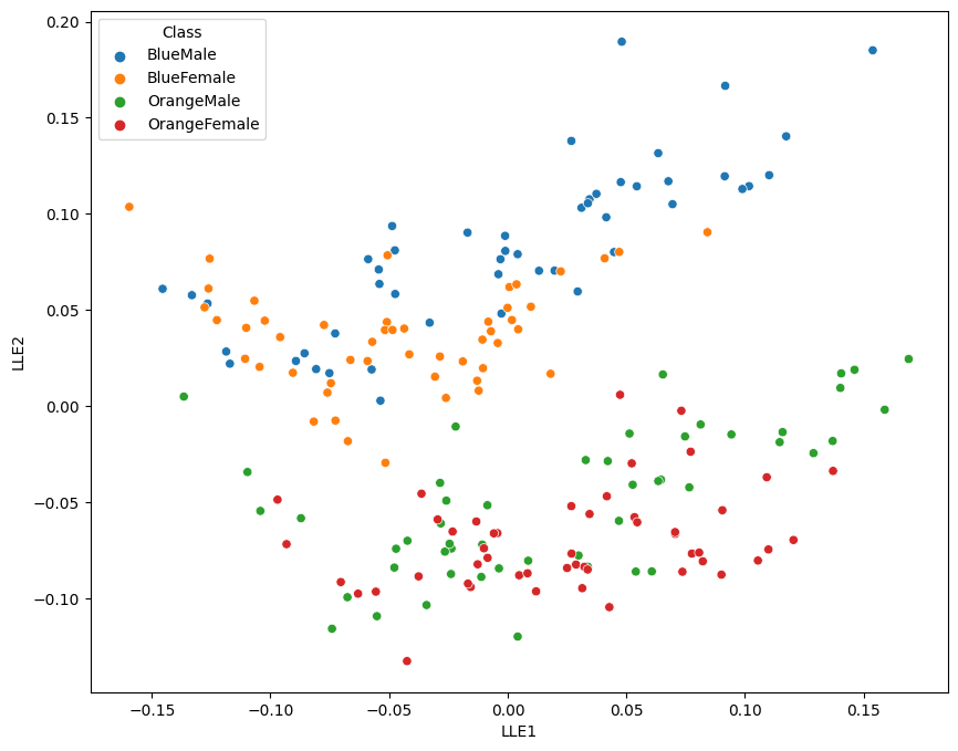
2-Dimensional Plot

fig = plt.figure(figsize=(10, 8))
sns.scatterplot(data=data_norm, x='LLE1', y='LLE2', hue='Class')

Already the 2d projection allows us to distinguish between the two species - Orange and Blue:

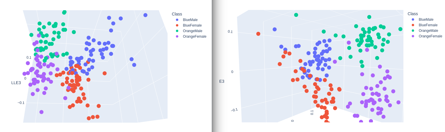
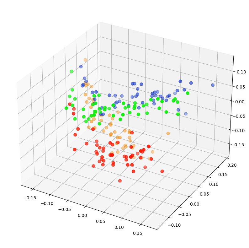
3-Dimensional Plot

class_colours = {
    'BlueMale': '#0027c4', #blue
    'BlueFemale': '#f18b0a', #orange
    'OrangeMale': '#0af10a', # green
    'OrangeFemale': '#ff1500', #red
}

colours = data['Class'].apply(lambda x: class_colours[x])

x=data_norm.LLE1
y=data_norm.LLE2
z=data_norm.LLE3

fig = plt.figure(figsize=(10,10))
ax = fig.add_subplot(projection='3d')

ax.scatter(xs=x, ys=y, zs=z, s=50, c=colours)

plot = px.scatter_3d(
    data_norm,
    x = 'LLE1',
    y = 'LLE2',
    z='LLE3',
    color='Class')

plot.show()