See also:
- Fun, fun, tensors: Tensor Constants, Variables and Attributes, Tensor Indexing, Expanding and Manipulations, Matrix multiplications, Squeeze, One-hot and Numpy
- Tensorflow 2 - Neural Network Regression: Building a Regression Model, Model Evaluation, Model Optimization, Working with a "Real" Dataset, Feature Scaling
- Tensorflow 2 - Neural Network Classification: Non-linear Data and Activation Functions, Model Evaluation and Performance Improvement, Multiclass Classification Problems
- Tensorflow 2 - Convolutional Neural Networks: Binary Image Classification, Multiclass Image Classification
- Tensorflow 2 - Transfer Learning: Feature Extraction, Fine-Tuning, Scaling
- Tensorflow 2 - Unsupervised Learning: Autoencoder Feature Detection, Autoencoder Super-Resolution, Generative Adverserial Networks
Tensorflow Neural Network Classification
Multiclass Classifications
Working with the MNIST Fashion Dataset -> 60k images / 10 classes
# importing the mnist dataset with keras
(train_data, train_labels), (test_data, test_labels) = tf.keras.datasets.fashion_mnist.load_data()
train_data.shape, test_data.shape
# ((60000, 28, 28), (10000, 28, 28)) => 60k training images & 10k testing images with 28x28px
# show example data

## training labels
class_names = ["T-shirt/Top", "Trousers", "Pullover", "Dress", "Coat", "Sandal", "Shirt", "Sneaker", "Bag", "Ankle Boot"]

## print label and data for index 666
print(f"Training Label:\n{class_names[train_labels[666]]}\n")
print(f"Training Data:\n{train_data[666]}")

plt.imshow(train_data[666], cmap=plt.cm.binary)
plt.title(class_names[train_labels[666]])

# Training Label:
# Sneaker

# Training Data:
# [[  0   0   0   0   0   0   0   0   0   0   0   0   0   0   0   0   0   0   0   0   0   0   0   0   0   0   0  0]
#  [  0   0   0   0   0   0   0   0   0   0   0   0   0   0   0   0   0   0   0   0   0   0   0   0   0   0   0  0]
#  [  0   0   0   0   0   0   0   0   0   0   0   0   0   0   0   0   0   0   0   0   0   0   0   0   0   0   0  0]
#  [  0   0   0   0   0   0   0   0   0   0   0   0   0   0   0   0   0   0   0   0   0   0   0   0   0   0   0  0]
#  [  0   0   0   0   0   0   0   0   0   0   0   0   0   0   0   0   0   0   0   0   0   0   0   0   0   0   0  0]
#  [  0   0   0   0   0   0   0   0   0   0   0   0   0   0   0   0   0   0   0   0   0   0   0   0   0   0   0  0]
#  [  0   0   0   0   0   0   0   0   0   0   0   0   0   0   0   0   0   0   0   0   0   0   0   0   0   0   0  0]
#  [  0   0   0   0   0   0   0   0   0   0   0   0   0   0   0   0   0   0   0   0   0   0   0   0   0   0   0  0]
#  [  0   0   0   0   0   0   0   0   0   0   0   2   0   0   0  25  51   0   5   0   0   0   0   0   0   0   0  0]
#  [  0   0   0   0   0   0   0   0   0   0   0   0   2  72  74 115 175   7   0   7   5   0   2   0 146 110   7  0]
#  [  0   0   0   0   0   0   0   0   0   0   0  54  95  92 123  77 123  72  20   0   0   0   0   0 255 136  51  0]
#  [  0   0   0   0   0   0   2   0   2  38  79  97 118  90 105 121  95 115  128  59  48   5   5  64 118 103  82 0]
#  [  0   0   0   0   0   5   2   0  61 121 108  92 115 162 167 162 175 133  105 113 144 133 110 133 144 146 141 2]
#  [  2   0   0   0   0   0   5  36 113 103  95 118 128 126 110 108 151 182  195 167 139 136 136 115 126 108 123 2]
#  [  0   0   2   0   7  33  51  85 105 123 128  92  90  79 108 133 103 121  162 170 193 206 151 126 123 123 118 5]
#  [  5  33  48  59  72  74  82  82 115 123 121 118 139 115  90 133 139 136  149 164 180 170 157 170 151 139 131 2]
#  [ 61 136 113  90  95  92 100 108 103 103 113 126 133 164 170 146 157 149  115  87  72  82 110 123 128 131 100 0]
#  [ 41  79 118 159 149 139 136 131 113 110 113 118 113  79  85  43  15  25  36  38  51  59  41  41  41  36  54  0]
#  [ 46  66  30  28  28  23  28  25  23  28  30  36  38  54  56  66  92 100  97  92  82  72  77  66  69  74  85 15]
#  [  0  20  54  69  72  72  79  82  79  82  79  82  82  72  82  87  74  72  74  64  54  54  56  51  56  54  51  7]
#  [  0   0   0   0   0   0   0   0   0   0   0   0   0   0   0   0   0   0  0   0   0   0   0   0   0   0   0   0]
#  [  0   0   0   0   0   0   0   0   0   0   0   0   0   0   0   0   0   0  0   0   0   0   0   0   0   0   0   0]
#  [  0   0   0   0   0   0   0   0   0   0   0   0   0   0   0   0   0   0  0   0   0   0   0   0   0   0   0   0]
#  [  0   0   0   0   0   0   0   0   0   0   0   0   0   0   0   0   0   0  0   0   0   0   0   0   0   0   0   0]
#  [  0   0   0   0   0   0   0   0   0   0   0   0   0   0   0   0   0   0  0   0   0   0   0   0   0   0   0   0]
#  [  0   0   0   0   0   0   0   0   0   0   0   0   0   0   0   0   0   0  0   0   0   0   0   0   0   0   0   0]
#  [  0   0   0   0   0   0   0   0   0   0   0   0   0   0   0   0   0   0  0   0   0   0   0   0   0   0   0   0]
#  [  0   0   0   0   0   0   0   0   0   0   0   0   0   0   0   0   0   0  0   0   0   0   0   0   0   0   0   0]]

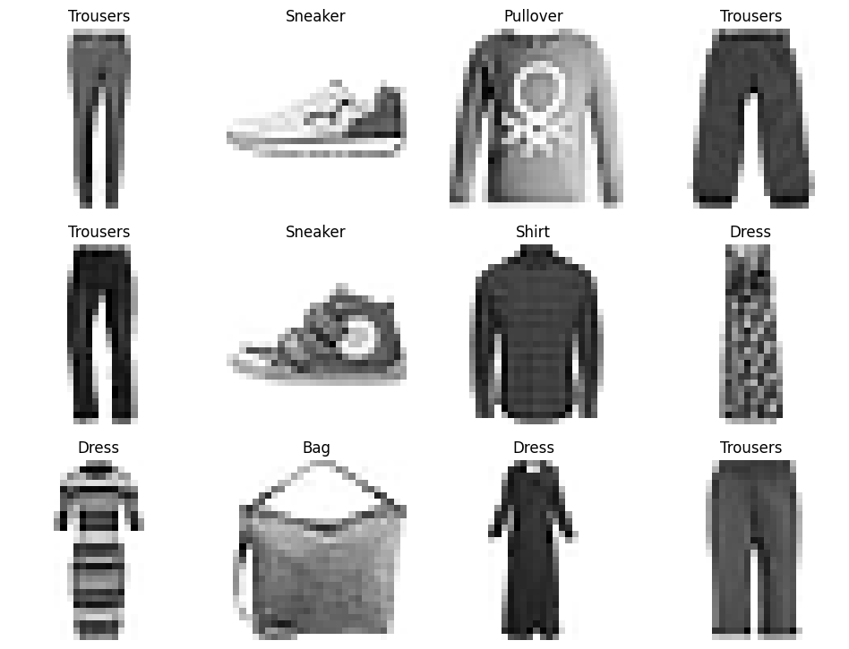
# plot multiple random images with labels
ran_gen = np.random.default_rng()

plt.figure(figsize=(12, 12))

for i in range(12):
    ax = plt.subplot(4, 4, i+1)
    random_index = ran_gen.integers(low=0, high=59999, size=1)
    plt.imshow(train_data[random_index[0]], cmap=plt.cm.binary)
    plt.title(class_names[train_labels[random_index[0]]])
    plt.axis(False)
Multiclass Classification Model
- Input Shape: Shape of the input image -> train_data[0].shape =
(28, 28) - Output Shape: Number of labels -> len(np.unique(train_labels)) =
10 - Loss Function:
tf.keras.losses.CategoricalCrossentropy - Output Layer Activation:
softmax
# determin the input and output shape
train_data[0].shape, len(np.unique(train_labels))
# ((28, 28), 10)
# building the model - 1st attempt
tf.random.set_seed(42)

model_multiclass = tf.keras.Sequential([
    tf.keras.layers.Dense(4, activation="relu", name="input_layer"),
    tf.keras.layers.Dense(4, activation="relu", name="dense_layer1"),
    tf.keras.layers.Dense(10, activation="softmax", name="output_layer")
])

model_multiclass.compile(loss=tf.keras.losses.CategoricalCrossentropy(),
                        optimizer=tf.keras.optimizers.Adam(learning_rate=0.0001),
                        metrics="accuracy")

history_multi = model_multiclass.fit(train_data, train_labels, batch_size=32,
                    validation_data=(test_data, test_labels),
                    epochs=100, verbose=1)

# ValueError: Shapes (32,) and (32, 28, 10) are incompatible
# => input data needs to be flattened
# building the model - 2nd attempt
tf.random.set_seed(42)

model_multiclass = tf.keras.Sequential([
    # flatten data from `28*28` => `None, 784`
    tf.keras.layers.Flatten(input_shape=(28, 28)),
    tf.keras.layers.Dense(4, activation="relu", name="input_layer"),
    tf.keras.layers.Dense(4, activation="relu", name="dense_layer1"),
    tf.keras.layers.Dense(10, activation="softmax", name="output_layer")
])

model_multiclass.compile(loss=tf.keras.losses.CategoricalCrossentropy(),
                        optimizer=tf.keras.optimizers.Adam(learning_rate=0.0001),
                        metrics="accuracy")

history_multi = model_multiclass.fit(train_data, train_labels, batch_size=32,
                    validation_data=(test_data, test_labels),
                    epochs=100, verbose=1)

# ValueError: Shapes (32, 1) and (32, 10) are incompatible
# => CategoricalCrossentropy() expects labels to be OneHot encoded
# use SparseCategoricalCrossentropy() instead
Use
SparseCategoricalCrossentropy()for "regular" labels
# building the model - 3rd attempt (works!)
tf.random.set_seed(42)

model_multiclass = tf.keras.Sequential([
    # flatten data from `28*28` to `None, 784`
    tf.keras.layers.Flatten(input_shape=(28, 28)),
    tf.keras.layers.Dense(4, activation="relu", name="input_layer"),
    tf.keras.layers.Dense(4, activation="relu", name="dense_layer1"),
    tf.keras.layers.Dense(10, activation="softmax", name="output_layer")
])

model_multiclass.compile(loss=tf.keras.losses.SparseCategoricalCrossentropy(),
                        optimizer=tf.keras.optimizers.Adam(learning_rate=0.0001),
                        metrics="accuracy")

history_multi = model_multiclass.fit(train_data, train_labels, batch_size=32,
                    validation_data=(test_data, test_labels),
                    epochs=100, verbose=1)

# Epoch 100/100
# 1875/1875 [==============================] - 3s 2ms/step - loss: 1.0307 - accuracy: 0.5697 - val_loss: 1.0820 - val_accuracy: 0.5568
Use
CategoricalCrossentropy()for OneHot encoded labels
# building the model - with OneHot encoded labels (alternative)
## OneHot encode labels
train_labels_hot = tf.one_hot(train_labels, depth=10)
test_labels_hot = tf.one_hot(test_labels, depth=10)

## re-run model with CategoricalCrossentropy() and ecoded labels
tf.random.set_seed(42)

model_multiclass_OneHot = tf.keras.Sequential([
    # flatten data from `28*28` to `None, 784`
    tf.keras.layers.Flatten(input_shape=(28, 28)),
    tf.keras.layers.Dense(4, activation="relu", name="input_layer"),
    tf.keras.layers.Dense(4, activation="relu", name="dense_layer1"),
    tf.keras.layers.Dense(10, activation="softmax", name="output_layer")
])

model_multiclass_OneHot.compile(loss=tf.keras.losses.CategoricalCrossentropy(),
                        optimizer=tf.keras.optimizers.Adam(learning_rate=0.0001),
                        metrics="accuracy")

history_multi_OneHot = model_multiclass_OneHot.fit(train_data, train_labels_hot, batch_size=32,
                    validation_data=(test_data, test_labels_hot),
                    epochs=100, verbose=1)

# Epoch 100/100
# 1875/1875 [==============================] - 4s 2ms/step - loss: 1.3885 - accuracy: 0.3996 - val_loss: 1.4322 - val_accuracy: 0.4055
Model Performance Improvements
model_multiclass.summary()

# Model: "sequential_1"
# _________________________________________________________________
#  Layer (type)                Output Shape              Param #
# =================================================================
#  flatten_1 (Flatten)         (None, 784)               0

#  input_layer (Dense)         (None, 4)                 3140

#  dense_layer1 (Dense)        (None, 4)                 20

#  output_layer (Dense)        (None, 10)                50

# =================================================================
# Total params: 3,210
# Trainable params: 3,210
# Non-trainable params: 0
# _________________________________________________________________
Normalize Data Inputs
The images are in grayscale and each pixel has a "dark level" between 0 and 255. We can use normalization to rearrange this scale to be between 0 and 1 instead. I do not expect there to be an advantage here. Normalization helps to make two features, that have different scales, comparable. Or in transfer learning - where the base model would, very likely, be trained on normalized data. So there should not be an effect here (?)
# check data value scale to verify
train_data.min(), train_data.max()
# (0, 255)
# the scaling here is simple - just divide by the maximum 255
train_data_norm = train_data / 255.0
test_data_norm = test_data / 255.0

# verify
train_data_norm.min(), train_data_norm.max(), test_data_norm.min(), test_data_norm.max()
# (0.0, 1.0, 0.0, 1.0)
# rebuild the model - this time with normalized data
tf.random.set_seed(42)
model_multiclass_norm = tf.keras.Sequential([
# flatten data from `28*28` to `None, 784`
tf.keras.layers.Flatten(input_shape=(28, 28)),
tf.keras.layers.Dense(4, activation="relu", name="input_layer"),
tf.keras.layers.Dense(4, activation="relu", name="dense_layer1"),
tf.keras.layers.Dense(10, activation="softmax", name="output_layer")
])
model_multiclass_norm.compile(loss=tf.keras.losses.SparseCategoricalCrossentropy(),
optimizer=tf.keras.optimizers.Adam(learning_rate=0.0001),
metrics="accuracy")
history_multi_norm = model_multiclass_norm.fit(train_data_norm, train_labels, batch_size=32,
validation_data=(test_data_norm, test_labels),
epochs=100, verbose=1)
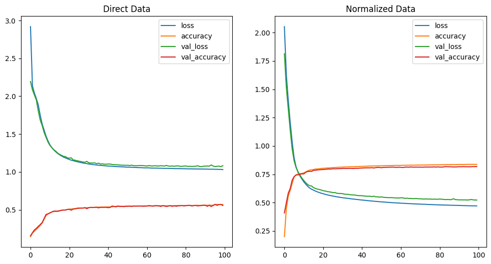
# oh wow - the loss is still quite high. but there is a big improvement in accuracy. unexpected...
# Epoch 100/100
# 1875/1875 [==============================] - 4s 2ms/step - loss: 0.4706 - accuracy: 0.8376 - val_loss: 0.5227 - val_accuracy: 0.8177
# print loss curves
fig, axes = plt.subplots(nrows=1, ncols=2, figsize=(12, 6))
pd.DataFrame(history_multi.history).plot(ax=axes[0], title="Direct Data")
pd.DataFrame(history_multi_norm.history).plot(ax=axes[1], title="Normalized Data")

# nomalized rules!
# confusion matrix
test_predictions = model_multiclass_norm.predict(test_data_norm)

confusion_norm = confusion_matrix(test_labels, np.argmax(test_predictions,axis=1))
confusion_norm

# the confusion matrix already  starts to look promising

# array([[757,   1,  27, 101,   4,   4,  85,   0,  19,   2],
#        [  3, 945,   9,  36,   5,   0,   1,   0,   1,   0],
#        [ 31,   3, 699,  10, 147,   0, 106,   0,   4,   0],
#        [ 49,  11,   8, 853,  28,   0,  41,   0,  10,   0],
#        [  1,   3, 111,  36, 738,   0, 102,   0,   9,   0],
#        [  0,   1,   0,   1,   0, 895,   0,  53,   3,  47],
#        [188,   4, 105,  62, 101,   0, 509,   0,  29,   2],
#        [  0,   0,   0,   0,   0,  42,   0, 926,   0,  32],
#        [  7,   2,   2,  11,   2,   4,  39,   5, 927,   1],
#        [  1,   0,   0,   0,   0,  18,   0,  52,   1, 928]])
Finding the Ideal Learning Rate
# add adaptive learning rate
tf.random.set_seed(42)

model_multiclass_norm_lr = tf.keras.Sequential([
    tf.keras.layers.Flatten(input_shape=(28, 28), name="input_layer"),
    tf.keras.layers.Dense(4, activation="relu", name="dense_layer1"),
    tf.keras.layers.Dense(4, activation="relu", name="dense_layer2"),
    tf.keras.layers.Dense(10, activation="softmax", name="output_layer")
])

model_multiclass_norm_lr.compile(loss=tf.keras.losses.SparseCategoricalCrossentropy(),
                                optimizer=tf.keras.optimizers.Adam(),
                                metrics=["accuracy"])

learning_rate_callback = tf.keras.callbacks.LearningRateScheduler(lambda epoch: 1e-4 * 10**(epoch/20))


model_multiclass_norm_lr_history = model_multiclass_norm_lr.fit(train_data_norm, train_labels,
                             callbacks=[learning_rate_callback],
                            validation_data=(test_data_norm, test_labels),
                            epochs=100, verbose=1)

# Epoch 100/100
# 1875/1875 [==============================] - 3s 2ms/step - loss: 3.1371 - accuracy: 0.0984 - val_loss: 2.4865 - val_accuracy: 0.1000 - lr: 8.9125
# get ideal learning rate by checking the lr decay curve
lr = 1e-4 * (10 ** (tf.range(100)/20))
plt.figure(figsize=(12, 7))
plt.title("Learning Rate Decay")
plt.xlabel("Learning Rate")
plt.ylabel("Loss")
plt.semilogx(lr, model_multiclass_norm_lr_history.history["loss"])
plt.show()
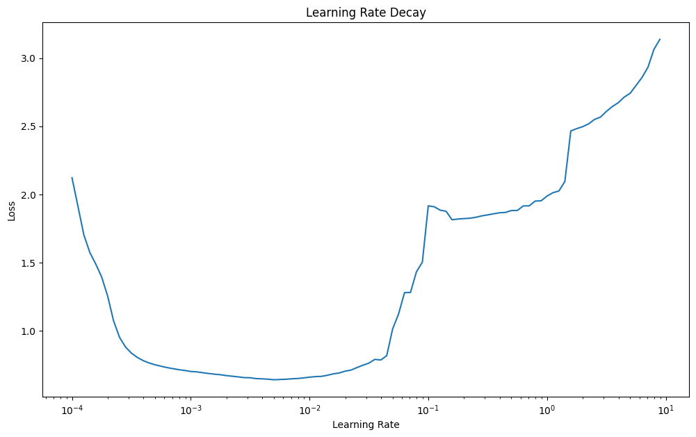
# the lowest point is at 4e-3 -> divide by 10
# the ideal learning rate is 4e-4 => model re-fit

tf.random.set_seed(42)

model_multiclass_norm = tf.keras.Sequential([
    # flatten data from `28*28` to `None, 784`
    tf.keras.layers.Flatten(input_shape=(28, 28)),
    tf.keras.layers.Dense(4, activation="relu", name="input_layer"),
    tf.keras.layers.Dense(4, activation="relu", name="dense_layer1"),
    tf.keras.layers.Dense(10, activation="softmax", name="output_layer")
])

model_multiclass_norm.compile(loss=tf.keras.losses.SparseCategoricalCrossentropy(),
                        optimizer=tf.keras.optimizers.Adam(learning_rate=4e-4),
                        metrics="accuracy")

history_multi_norm = model_multiclass_norm.fit(train_data_norm, train_labels, batch_size=32,
                    validation_data=(test_data_norm, test_labels),
                    epochs=100, verbose=1)

# Epoch 100/100
# 1875/1875 [==============================] - 4s 2ms/step - loss: 0.5323 - accuracy: 0.8042 - val_loss: 0.6132 - val_accuracy: 0.7862
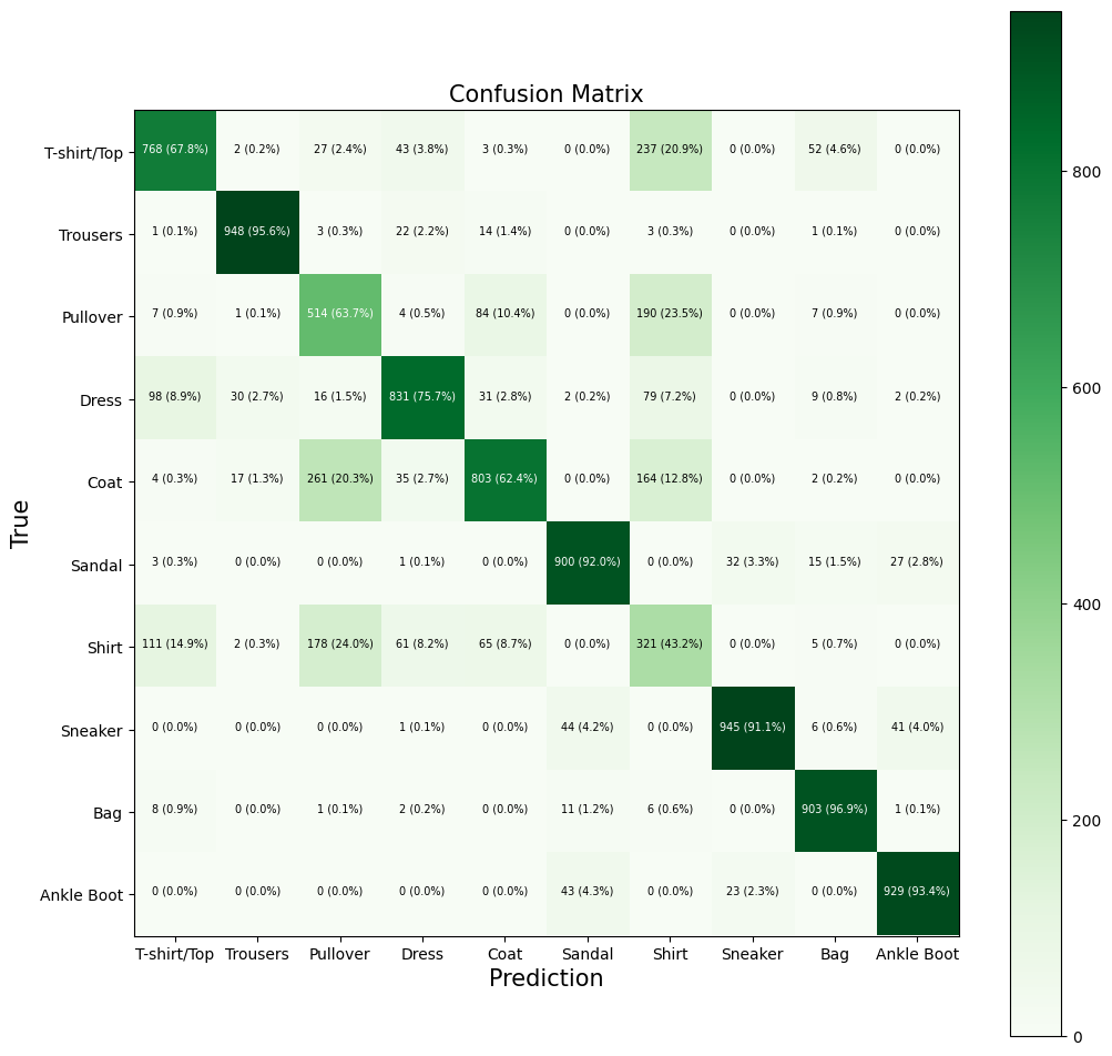
# plot confusion matrix
import itertools

def plot_confusion_matrix(y_pred, y_true, classes=None, figsize = (12, 12), text_size=7):

        # create the confusion matrix
        cm = confusion_matrix(y_pred, y_true)

        # normalize
        cm_norm = cm.astype("float") / cm.sum(axis=1)[:, np.newaxis]
        # cm_norm
        # array([[1., 0.],
        #        [0., 1.]])

        number_of_classes = cm.shape[0]
        # 2

        # plot matrix
        fig, ax = plt.subplots(figsize=figsize)
        cax = ax.matshow(cm, cmap=plt.cm.Greens)
        fig.colorbar(cax)

        if classes:
            labels = classes
        else:
            labels = np.arange(cm.shape[0])

        # axes lables
        ax.set(title="Confusion Matrix",
              xlabel="Prediction",
              ylabel="True",
              xticks=np.arange(number_of_classes),
              yticks=np.arange(number_of_classes),
              xticklabels=labels,
              yticklabels=labels)

        ax.xaxis.set_label_position("bottom")
        ax.title.set_size(15)
        ax.xaxis.label.set_size(15)
        ax.yaxis.label.set_size(15)
        ax.xaxis.tick_bottom()


        # colour threshold
        threshold = (cm.max() + cm.min()) / 2.

        # add text to cells
        for i, j in itertools.product(range(cm.shape[0]), range(cm.shape[1])):
            plt.text(j, i , f"{cm[i, j]} ({cm_norm[i, j]*100:.1f}%)",
            horizontalalignment="center",
            color="white" if cm[i, j] > threshold else "black",
            size=text_size)
## start by running predictions on the test dataset
test_predictions_ideal = model_multiclass_norm.predict(test_data_norm)
## set class with highest probability to 1 - rest to zero
y_pred = tf.argmax(test_predictions_ideal,axis=1)
## plot the confusion matrix predictions vs true labels
plot_confusion_matrix(y_pred=y_pred, y_true=test_labels, classes=class_names)
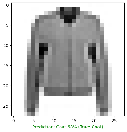
Making predictions to further evaluate the model
# function to pick a random image and run prediction
def random_image_prediction(model, images, true_labels, classes):
    # create random image index
    i = random.randint(0, len(images))
    # select label of image at index i
    true_label = classes[true_labels[i]]
    # pick corresponding image
    target_image = images[i]
    # reshape image and pass it to prediction
    pred_probabilities = model.predict(target_image.reshape(1, 28, 28))
    # select class with highest probability
    pred_label = classes[pred_probabilities.argmax()]

    # plot the b&w image
    plt.imshow(target_image, cmap=plt.cm.binary)

    if pred_label == true_label:
        color = "green"
    else:
        color = "red"

    plt.xlabel("Prediction: {} {:2.0f}% (True: {})".format(pred_label,
                                                     100*tf.reduce_max(pred_probabilities),
                                                     true_label), color = color)
random_image_prediction(model=model_multiclass_norm,
                       images=test_data_norm,
                       true_labels=test_labels,
                       classes=class_names)
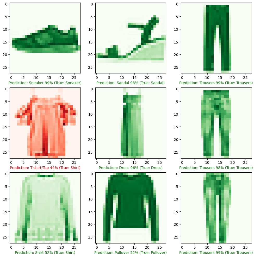
# function to pick a random image and run prediction
def random_image_map_prediction(model, images, true_labels, classes):

    ran_gen = np.random.default_rng()

    plt.figure(figsize=(12, 12))

    for i in range(9):
        # select random image
        random_index = ran_gen.integers(low=0, high=len(images), size=1)
        target_image = images[random_index[0]]
        true_label = classes[true_labels[random_index[0]]]
        # reshape image and pass it to prediction
        pred_probabilities = model.predict(target_image.reshape(1, 28, 28))
        # select class with highest probability
        pred_label = classes[pred_probabilities.argmax()]

        ax = plt.subplot(3, 3, i+1)
        # plt.title(classes[train_labels[random_index[0]]])

        if pred_label == true_label:
            colour = "green"
            colourmap = "Greens"
        else:
            colour = "red"
            colourmap = "Reds"

        plt.xlabel("Prediction: {} {:2.0f}% (True: {})".format(pred_label,
                                                         100*tf.reduce_max(pred_probabilities),
                                                         true_label), color = colour)
        plt.imshow(target_image, cmap=colourmap)
        plt.axis(True)
random_image_map_prediction(model=model_multiclass_norm,
                       images=test_data_norm,
                       true_labels=test_labels,
                       classes=class_names)
Weights & Biases
Weights represent the pattern a particular layer of our neural network has learned during training.
model_multiclass_norm.layers

# [<keras.layers.reshaping.flatten.Flatten at 0x7f0e24157940>,
#   <keras.layers.core.dense.Dense at 0x7f0e2423e560>,
#   <keras.layers.core.dense.Dense at 0x7f0eedc336d0>,
#   <keras.layers.core.dense.Dense at 0x7f0e2423e620>]
# get weigths of a particular layer
weights, biases = model_multiclass_norm.layers[1].get_weights()

weights.shape, weights, biases.shape, biases, model_multiclass_norm.summary()

# weight.shape
#  (784, 4)) => 28x28 for the image dimensions and 4 hidden units

# weights
# (array([[-1.3565315 , -0.3214511 , -0.16312897, -0.3301181 ],
#         [-1.8619745 ,  0.22111109, -1.3103486 ,  1.1400424 ],
#         [ 1.9727688 , -1.762827  , -1.5388335 ,  0.39442703],
#         ...,
#         [ 0.5418353 ,  0.5226571 ,  0.27219778,  0.4796965 ],
#         [-0.55814236,  0.2910452 ,  0.26502737,  2.1195614 ],
#         [-0.5417867 , -0.16617213,  1.1190995 ,  0.3001483 ]],
#        dtype=float32)
# for every pixel in our sample 28x28px images we get 4 different
# values from the 4 hidden units / neurons inspecting the image for features
# weights

# biases.shape => for every hidden unit we get a bias vector
# (4,),

# biases => dictate how much the corresponding weight should influence the next layer
#  array([ 1.9621418 ,  0.5325201 ,  1.6395437 , -0.04142712], dtype=float32),
#  None)

# model summary
# Model: "sequential_1"
# _________________________________________________________________
#  Layer (type)                Output Shape              Param #
# =================================================================
#  flatten_1 (Flatten)         (None, 784)               0

#  input_layer (Dense)         (None, 4)                 3140

#  dense_layer1 (Dense)        (None, 4)                 20

#  output_layer (Dense)        (None, 10)                50

# =================================================================
# Total params: 3,210
# Trainable params: 3,210
# Non-trainable params: 0
# _________________________________________________________________