• Detection of Exoplanets using Transit Photometry
  • Dataset Preprocessing
    • Missing Values
    • Label Imbalance
    • Visualizing Differences between both Classes
    • Handling Outliers
  • Model Training
    • KNN Model on Imbalanced Datasets
    • Model Evaluation
    • Random Oversampling to balance the Dataset
    • KNN Model on the balanced Data
    • Model Evaluation
    • Hyper Parameter Tuning
  • AutoML with AutoGluon
    • Tabular Data Predictor on the unbalanced Dataset
      • Data Preprocessing
      • Model Training
      • Model Evaluation
    • Tabular Data Predictor on the re-balanced Dataset
      • Data Preprocessing
      • Model Training
      • Model Evaluation
    • Multi Modal Predictor on the re-balanced Dataset
      • Data Preprocessing
      • Model Training
      • Model Evaluation

Github Repository

Detection of Exoplanets using Transit Photometry

Detection of exoplanets using transit photometry:

• Sky Debnath: Department of Physics, National Institute of Technology Agartala, Jirania, West Tripura, Tripura 799046
• Avinash A Deshpande: Astronomy and Astrophysics, Raman Research Institute, C. V. Raman Avenue, Sadashivnagar, Bengaluru 560080

images source

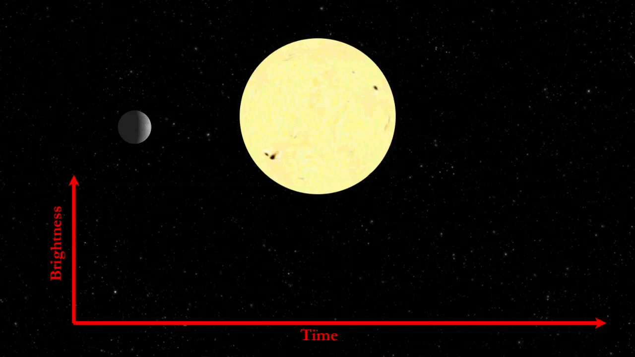
Exoplanets are the planets found outside of the solar system. When a planet passes in front of a star, the brightness of that star as observed by us becomes dimmer depending on the size of the planet. The data we observe will show a dip in flux if a planet is transiting the star we are observing.

Dataset: Exoplanet Hunting in Deep Space - Kepler labelled time series data.

The data describe the change in flux (light intensity) of several thousand stars. Each star has a binary label of 2 or 1. 2 indicated that that the star is confirmed to have at least one exoplanet in orbit

from autogluon.multimodal import MultiModalPredictor
from autogluon.tabular import TabularDataset, TabularPredictor
from imblearn.over_sampling import RandomOverSampler
import numpy as np
import matplotlib.pyplot as plt
import pandas as pd
import seaborn as sns
from sklearn.metrics import (
    confusion_matrix,
    ConfusionMatrixDisplay,
    accuracy_score,
    classification_report
)
from sklearn.model_selection import train_test_split, GridSearchCV
from sklearn.neighbors import KNeighborsClassifier as KNC
from sklearn.preprocessing import StandardScaler
plt.style.use('fivethirtyeight')

SEED=42
MODEL_PATH = 'model'

Dataset Preprocessing

df_train = pd.read_csv('dataset/exoTrain.csv')
df_test = pd.read_csv('dataset/exoTest.csv')

print(df_train.shape, df_test.shape)
# (5087, 3198) (570, 3198)

df_train.head(5).transpose()

	0	1	2	3	4
LABEL	2.00	2.00	2.00	2.00	2.00
FLUX.1	93.85	-38.88	532.64	326.52	-1107.21
FLUX.2	83.81	-33.83	535.92	347.39	-1112.59
FLUX.3	20.10	-58.54	513.73	302.35	-1118.95
FLUX.4	-26.98	-40.09	496.92	298.13	-1095.10
...
FLUX.3193	92.54	0.76	5.06	-12.67	-438.54
FLUX.3194	39.32	-11.70	-11.80	-8.77	-399.71
FLUX.3195	61.42	6.46	-28.91	-17.31	-384.65
FLUX.3196	5.08	16.00	-70.02	-17.35	-411.79
FLUX.3197	-39.54	19.93	-96.67	13.98	-510.54

# replacing label class [1,2] -> [0,1]
df_train = df_train.replace({'LABEL': {2:1, 1:0}})
df_test = df_test.replace({'LABEL': {2:1, 1:0}})

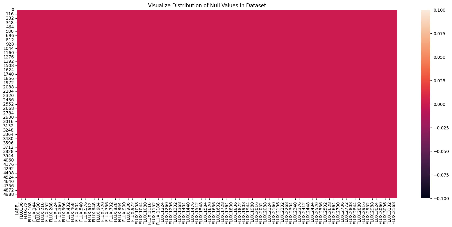
Missing Values

# how many values are missing?
print(df_train.isnull().sum().sum())
# 0 => no missing data
plt.figure(figsize=(20, 8))
plt.title('Visualize Distribution of Null Values in Dataset')

sns.heatmap(
    df_train.isnull(),
    annot=False
)

plt.savefig('assets/Real_World_Model_to_Deployment_01.webp', bbox_inches='tight')

Label Imbalance

# is the dataset balanced?
df_train['LABEL'].value_counts()

# the dataset only has 37 positives against 5050 negatives
# 0    5050
# 1      37
# Name: LABEL, dtype: int64

plt.figure(figsize=(10, 5))
plt.title('Suns w/o (Class 0) and w (Class 1) Exoplanets')

ax = sns.countplot(
    data=df_train,
    x='LABEL'
)

ax.bar_label(ax.containers[0])

plt.savefig('assets/Real_World_Model_to_Deployment_02.webp', bbox_inches='tight')

exoplanets = df_train[df_train['LABEL'] == 1.]
exoplanets

	LABEL	FLUX.1	FLUX.2	FLUX.3	FLUX.4	FLUX.5	FLUX.6	FLUX.7	FLUX.8	FLUX.9	...	FLUX.3188	FLUX.3189	FLUX.3190	FLUX.3191	FLUX.3192	FLUX.3193	FLUX.3194	FLUX.3195	FLUX.3196	FLUX.3197
0	1	93.85	83.81	20.10	-26.98	-39.56	-124.71	-135.18	-96.27	-79.89	...	-78.07	-102.15	-102.15	25.13	48.57	92.54	39.32	61.42	5.08	-39.54
1	1	-38.88	-33.83	-58.54	-40.09	-79.31	-72.81	-86.55	-85.33	-83.97	...	-3.28	-32.21	-32.21	-24.89	-4.86	0.76	-11.70	6.46	16.00	19.93
2	1	532.64	535.92	513.73	496.92	456.45	466.00	464.50	486.39	436.56	...	-71.69	13.31	13.31	-29.89	-20.88	5.06	-11.80	-28.91	-70.02	-96.67
3	1	326.52	347.39	302.35	298.13	317.74	312.70	322.33	311.31	312.42	...	5.71	-3.73	-3.73	30.05	20.03	-12.67	-8.77	-17.31	-17.35	13.98
4	1	-1107.21	-1112.59	-1118.95	-1095.10	-1057.55	-1034.48	-998.34	-1022.71	-989.57	...	-594.37	-401.66	-401.66	-357.24	-443.76	-438.54	-399.71	-384.65	-411.79	-510.54
5	1	211.10	163.57	179.16	187.82	188.46	168.13	203.46	178.65	166.49	...	-98.45	30.34	30.34	29.62	28.80	19.27	-43.90	-41.63	-52.90	-16.16
6	1	9.34	49.96	33.30	9.63	37.64	20.85	4.54	22.42	10.11	...	-58.56	9.93	9.93	23.50	5.28	-0.44	10.90	-11.77	-9.25	-36.69
7	1	238.77	262.16	277.80	190.16	180.98	123.27	103.95	50.70	59.91	...	-72.48	31.77	31.77	53.48	27.88	95.30	48.86	-10.62	-112.02	-229.92
8	1	-103.54	-118.97	-108.93	-72.25	-61.46	-50.16	-20.61	-12.44	1.48	...	43.92	7.24	7.24	-7.45	-18.82	4.53	21.95	26.94	34.08	44.65
9	1	-265.91	-318.59	-335.66	-450.47	-453.09	-561.47	-606.03	-712.72	-685.97	...	3671.03	2249.28	2249.28	2437.78	2584.22	3162.53	3398.28	3648.34	3671.97	3781.91
10	1	118.81	110.97	79.53	114.25	48.78	3.12	-4.09	66.20	-26.02	...	50.05	50.05	50.05	67.42	-56.78	126.14	200.36	432.95	721.81	938.08
11	1	-239.88	-164.28	-180.91	-225.69	-90.66	-130.66	-149.75	-120.50	-157.00	...	-364.75	-364.75	-364.75	-196.38	-165.81	-215.94	-293.25	-214.34	-154.84	-151.41
12	1	70.34	63.86	58.37	69.43	64.18	52.70	47.58	46.89	46.00	...	6.45	-8.91	-8.91	-6.70	-5.04	-10.79	-4.97	-7.46	-15.06	-2.06
13	1	424.14	407.71	461.59	428.17	412.69	395.58	453.35	410.45	402.09	...	238.36	46.65	46.65	95.90	123.48	138.38	190.66	202.55	232.16	251.73
14	1	-267.21	-239.11	-233.15	-211.84	-191.56	-181.69	-164.77	-156.68	-139.23	...	-754.92	-752.38	-752.38	-754.93	-761.64	-746.83	-765.22	-757.05	-763.26	-769.39
15	1	35.92	45.84	47.99	74.58	87.97	87.97	105.23	131.70	130.00	...	39.71	-2.53	-2.53	15.32	18.65	20.43	22.40	37.32	36.01	71.59
16	1	-122.30	-122.30	-131.08	-109.69	-109.69	-95.27	-93.93	-84.84	-73.65	...	22.64	-42.53	-42.53	-46.43	-56.26	-54.25	-37.13	-24.73	13.35	-5.81
17	1	-65.20	-76.33	-76.23	-72.58	-69.62	-74.51	-69.48	-61.06	-49.29	...	18.66	-11.72	-11.72	4.56	11.47	31.26	21.71	13.42	13.24	9.21
18	1	-66.47	-15.50	-44.59	-49.03	-70.16	-85.53	-52.06	-73.41	-59.69	...	-6.19	10.00	10.00	50.12	-14.97	-32.75	-30.28	-9.28	-31.53	26.88
19	1	560.19	262.94	189.94	185.12	210.38	104.19	289.56	172.06	81.75	...	106.00	-7.94	-7.94	-7.94	52.31	-165.00	7.38	-61.56	-44.75	104.50
20	1	-1831.31	-1781.44	-1930.84	-2016.72	-1963.31	-1956.12	-2128.24	-2188.20	-2212.82	...	903.82	75.61	75.61	191.77	196.16	326.61	481.28	635.63	651.68	695.74
21	1	2053.62	2126.05	2146.33	2159.84	2237.59	2236.12	2244.47	2279.61	2288.22	...	1832.59	1935.53	1965.84	2094.19	2212.52	2292.64	2454.48	2568.16	2625.45	2578.80
22	1	-48.48	-22.95	11.15	-70.04	-120.34	-150.04	-309.38	-160.73	-201.41	...	90.70	-20.01	-62.12	-45.96	-52.40	-4.93	26.74	21.43	145.30	197.20
23	1	145.84	137.82	96.99	17.09	-73.79	-157.79	-267.71	-365.91	-385.07	...	62.76	101.24	98.13	112.51	95.77	127.98	67.51	91.24	40.40	-10.80
24	1	207.37	195.04	150.45	135.34	104.90	59.79	42.85	52.74	18.38	...	-13.21	-43.43	-14.77	-22.27	-0.04	19.46	9.32	23.55	-4.73	11.82
25	1	304.50	275.94	269.24	248.51	194.88	167.80	139.13	149.36	100.97	...	4.21	3.53	-5.13	14.56	-1.44	-10.73	3.49	0.18	-2.89	40.34
26	1	150725.80	129578.36	102184.98	82253.98	67934.17	48063.52	42745.02	18971.55	2983.58	...	-11143.45	-23351.45	-33590.27	-31861.95	-23298.89	-13056.11	379.48	9444.52	23261.02	33565.48
27	1	124.39	72.73	36.85	-4.68	6.96	-44.61	-89.79	-121.71	-120.59	...	-14.38	-21.65	-6.04	-7.15	67.58	56.43	-1.95	7.09	1.63	-10.77
28	1	-63.50	-49.15	-45.99	-34.55	-44.34	-15.80	-16.07	5.32	-7.05	...	-113.73	-113.58	-130.99	-121.51	-94.69	-90.38	-74.36	-56.49	-46.51	-44.53
29	1	31.29	25.14	36.93	16.63	17.01	-7.50	0.09	1.24	-19.82	...	11.36	12.96	28.50	51.05	25.85	4.79	13.26	-17.58	13.79	0.72
30	1	-472.50	-384.09	-330.42	-273.41	-185.02	-115.64	-141.86	-16.23	77.80	...	-3408.88	-3425.92	-3465.59	-3422.95	-3398.83	-3410.42	-3393.58	-3407.78	-3391.56	-3397.03
31	1	194.82	162.51	126.17	129.70	82.27	60.71	58.71	23.36	32.57	...	29.21	47.66	0.48	-28.59	-33.15	-14.98	-1.56	22.25	21.55	3.49
32	1	26.96	38.98	25.99	47.28	26.29	34.08	16.66	28.27	20.99	...	35.26	-9.94	23.73	-7.54	-5.86	13.04	-5.64	-16.85	-6.18	-16.03
33	1	43.07	46.73	29.43	9.75	6.54	-3.76	-31.48	-46.94	-40.78	...	6.99	5.75	23.18	15.08	18.09	13.40	15.78	18.18	51.21	9.71
34	1	-248.23	-243.59	-217.91	-190.69	-190.17	-163.04	-196.32	-164.73	-149.34	...	94.25	121.45	135.02	147.14	161.89	198.05	262.03	282.88	334.81	377.14
35	1	22.82	46.37	39.61	98.75	81.32	100.43	65.00	38.86	22.11	...	55.50	-16.22	-5.21	15.04	11.86	-5.38	-24.46	-55.86	-44.55	-16.80
36	1	26.24	42.32	28.34	24.81	49.39	47.57	41.52	51.80	25.50	...	-7.53	-35.72	-14.32	-29.21	-30.61	8.49	4.75	6.59	-7.03	24.41

37 rows × 3198 columns

Visualizing Differences between both Classes

# separate label
X_train = df_train.drop(['LABEL'], axis=1)
y_train = df_train['LABEL']
X_test = df_test.drop(['LABEL'], axis=1)
y_test = df_test['LABEL']

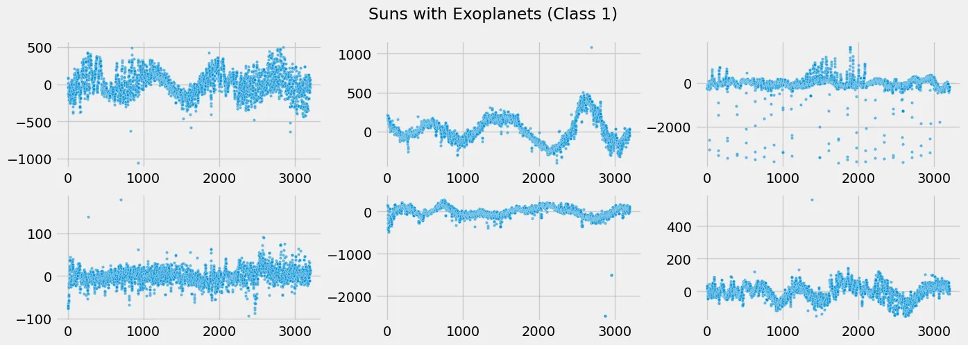
# plot light curve for a single sun
## there are no timestamp -> generate range
time = range(1,3198)
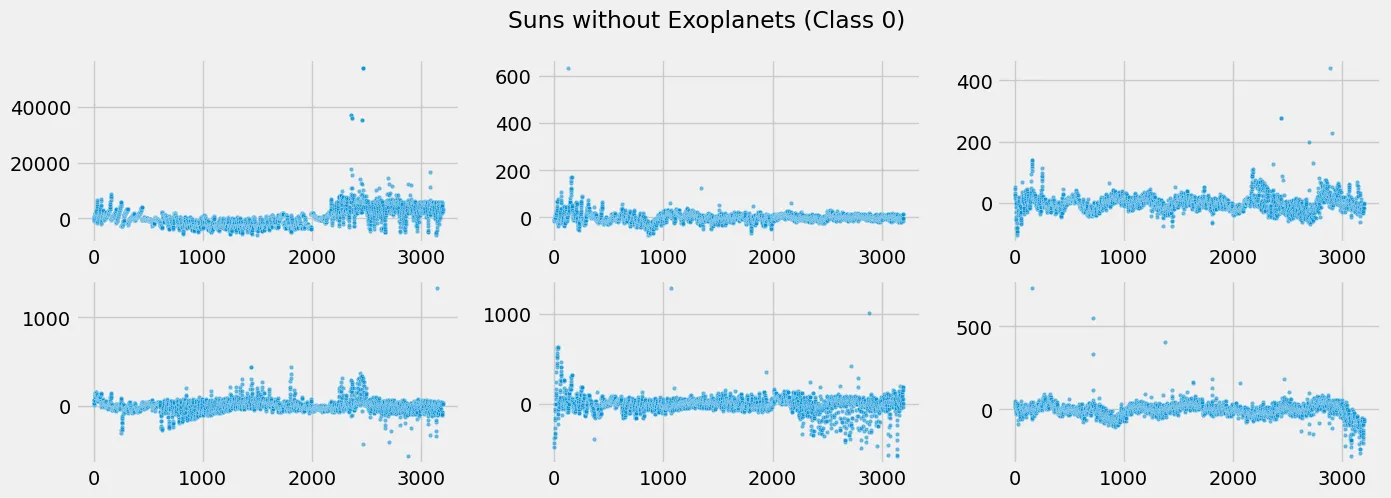
## get brightness values for suns (class 0)
flux_00 = X_train.iloc[444,:].values
flux_01 = X_train.iloc[222,:].values
flux_02 = X_train.iloc[666,:].values
flux_03 = X_train.iloc[888,:].values
flux_04 = X_train.iloc[111,:].values
flux_05 = X_train.iloc[5000,:].values
## get brightness values for suns (class 1)
flux_10 = X_train.iloc[0,:].values
flux_11 = X_train.iloc[5,:].values
flux_12 = X_train.iloc[11,:].values
flux_13 = X_train.iloc[17,:].values
flux_14 = X_train.iloc[23,:].values
flux_15 = X_train.iloc[29,:].values

fig, axes = plt.subplots(2, 3, figsize=(15, 5))
fig.suptitle('Suns with Exoplanets (Class 1)')

sns.scatterplot(
    x=time,
    y=flux_10,
    s=10,
    alpha=0.6,
    ax=axes[0,0]
)

sns.scatterplot(
    x=time,
    y=flux_11,
    s=10,
    alpha=0.6,
    ax=axes[0,1]
)

sns.scatterplot(
    x=time,
    y=flux_12,
    s=10,
    alpha=0.6,
    ax=axes[0,2]
)

sns.scatterplot(
    x=time,
    y=flux_13,
    s=10,
    alpha=0.6,
    ax=axes[1,0]
)

sns.scatterplot(
    x=time,
    y=flux_14,
    s=10,
    alpha=0.6,
    ax=axes[1,1]
)

sns.scatterplot(
    x=time,
    y=flux_15,
    s=10,
    alpha=0.6,
    ax=axes[1,2]
)

plt.savefig('assets/Real_World_Model_to_Deployment_03.webp', bbox_inches='tight')

fig, axes = plt.subplots(2, 3, figsize=(15, 5))
fig.suptitle('Suns without Exoplanets (Class 0)')

sns.scatterplot(
    x=time,
    y=flux_00,
    s=10,
    alpha=0.6,
    ax=axes[0,0]
)

sns.scatterplot(
    x=time,
    y=flux_01,
    s=10,
    alpha=0.6,
    ax=axes[0,1]
)

sns.scatterplot(
    x=time,
    y=flux_02,
    s=10,
    alpha=0.6,
    ax=axes[0,2]
)

sns.scatterplot(
    x=time,
    y=flux_03,
    s=10,
    alpha=0.6,
    ax=axes[1,0]
)

sns.scatterplot(
    x=time,
    y=flux_04,
    s=10,
    alpha=0.6,
    ax=axes[1,1]
)

sns.scatterplot(
    x=time,
    y=flux_05,
    s=10,
    alpha=0.6,
    ax=axes[1,2]
)

plt.savefig('assets/Real_World_Model_to_Deployment_04.webp', bbox_inches='tight')

Handling Outliers

plt.figure(figsize=(15, 5))

for i in range(1,5):
    plt.subplot(1,4,i)
    sns.boxplot(data=df_train, x='LABEL', y='FLUX.' + str(i))

plt.savefig('assets/Real_World_Model_to_Deployment_05.webp', bbox_inches='tight')

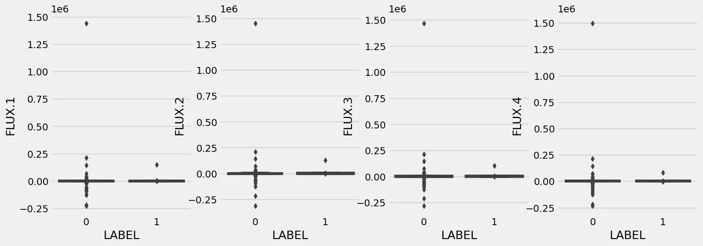
# there is one extreme outlier with a value above 0.25e6 in FLUX.1
df_train[df_train['FLUX.1'] > 0.25e6].index
# Int64Index([3340], dtype='int64')

df_train[df_train['FLUX.3'] > 0.25e6].index
# Int64Index([3340], dtype='int64')

# it is the same sun in both cases with iloc 3340 -> drop
df_train = df_train.drop(3340, axis=0)

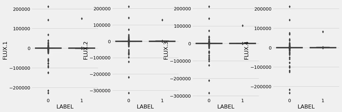
plt.figure(figsize=(15, 5))

for i in range(1,5):
    plt.subplot(1,4,i)
    sns.boxplot(data=df_train, x='LABEL', y='FLUX.' + str(i))

plt.savefig('assets/Real_World_Model_to_Deployment_06.webp', bbox_inches='tight')

Model Training

# the dataset is already split into train/test -> further split validation from train set
X_train, X_val, y_train, y_val = train_test_split(
    X_train, y_train, test_size=0.3, random_state=SEED
)

X_train.shape, X_val.shape
# ((3560, 3197), (1527, 3197))

# normalizing features
scaler = StandardScaler()
X_train_scaled = scaler.fit_transform(X_train)
X_test_scaled = scaler.fit_transform(X_test)
X_val_scaled = scaler.fit_transform(X_val)

KNN Model on Imbalanced Datasets

knn_classifier = KNC(n_neighbors=5, metric='minkowski', p=2)

knn_classifier.fit(X_train_scaled, y_train)

Model Evaluation

y_pred = knn_classifier.predict(X_val)
print(accuracy_score(y_pred, y_val))
# 0.9921414538310412
print(classification_report(y_val, y_pred))
# the imbalanced dataset leads to spectacular accuracies, but...

	precision	recall	f1-score	support
0	0.99	1.00	1.00	1515
1	0.00	0.00	0.00	12
accuracy			0.99	1527
macro avg	0.50	0.50	0.50	1527
weighted avg	0.98	0.99	0.99	1527

# because there are so few positives in the dataset
# the accuracy is not affected by a 100% fail in detection
ConfusionMatrixDisplay(
    confusion_matrix=confusion_matrix(y_val, y_pred)
).plot()

plt.savefig('assets/Real_World_Model_to_Deployment_07.webp', bbox_inches='tight')

Random Oversampling to balance the Dataset

# get full training dataset again
X_train = df_train.drop(['LABEL'], axis=1)
y_train = df_train['LABEL']

over_sampler = RandomOverSampler()

x_osample, y_osample =over_sampler.fit_resample(X_train, y_train)

plt.figure(figsize=(10, 5))
plt.title('Suns w/o (Class 0) and w (Class 1) Exoplanets')

ax = y_osample.value_counts().plot(kind='bar')
ax.bar_label(ax.containers[0])

plt.savefig('assets/Real_World_Model_to_Deployment_08.webp', bbox_inches='tight')

KNN Model on the balanced Data

# the dataset is already split into train/test -> further split validation from train set
X_train, X_val, y_train, y_val = train_test_split(
    x_osample, y_osample, test_size=0.3, random_state=SEED
)

X_train.shape, X_val.shape
# ((7068, 3197), (3030, 3197))

# normalizing features
scaler = StandardScaler()
X_train_scaled = scaler.fit_transform(X_train)
X_val_scaled = scaler.fit_transform(X_val)

knn_classifier = KNC(n_neighbors=5, metric='minkowski', p=2)

knn_classifier.fit(X_train_scaled, y_train)

Model Evaluation

y_pred = knn_classifier.predict(X_val)
print(accuracy_score(y_pred, y_val))
# 0.6026402640264027
print(classification_report(y_val, y_pred))

	precision	recall	f1-score	support
0	0.57	0.94	0.71	1558
1	0.80	0.24	0.37	1472
accuracy			0.60	3030
macro avg	0.68	0.59	0.54	3030
weighted avg	0.68	0.60	0.55	3030

ConfusionMatrixDisplay(
    confusion_matrix=confusion_matrix(y_val, y_pred)
).plot()

plt.savefig('assets/Real_World_Model_to_Deployment_09.webp', bbox_inches='tight')

Hyper Parameter Tuning

knn_classifier = KNC()

param_grid = {
    'n_neighbors': [4, 5, 6],
    'weights': ['uniform', 'distance'],
    'p': [1, 2]
}

grid_search = GridSearchCV(
    estimator = knn_classifier,
    param_grid = param_grid
)

grid_search.fit(X_train_scaled, y_train)

print('Best Parameter: ', grid_search.best_params_)
# Best Parameter:  {'n_neighbors': 4, 'p': 2, 'weights': 'uniform'}

# re-run training with new
knn_classifier = KNC(n_neighbors=4, metric='minkowski', p=2, weights='uniform')
knn_classifier.fit(X_train_scaled, y_train)

y_pred = knn_classifier.predict(X_val)
print(accuracy_score(y_pred, y_val))
# 0.5712871287128712
print(classification_report(y_val, y_pred))

	precision	recall	f1-score	support
0	0.55	0.96	0.70	1558
1	0.81	0.15	0.26	1472
accuracy			0.57	3030
macro avg	0.68	0.56	0.48	3030
weighted avg	0.67	0.57	0.49	3030

ConfusionMatrixDisplay(
    confusion_matrix=confusion_matrix(y_val, y_pred)
).plot()

plt.savefig('assets/Real_World_Model_to_Deployment_10.webp', bbox_inches='tight')

AutoML with AutoGluon

Tabular Data Predictor on the unbalanced Dataset

Data Preprocessing

data = TabularDataset('dataset/exoTrain.csv')
# replacing label class [1,2] -> [0,1]
data = data.replace({'LABEL': {2:1, 1:0}})
data.head(5).transpose()

	0	1	2	3	4
LABEL	1.00	1.00	1.00	1.00	1.00
FLUX.1	93.85	-38.88	532.64	326.52	-1107.21
FLUX.2	83.81	-33.83	535.92	347.39	-1112.59
FLUX.3	20.10	-58.54	513.73	302.35	-1118.95
FLUX.4	-26.98	-40.09	496.92	298.13	-1095.10
...
FLUX.3193	92.54	0.76	5.06	-12.67	-438.54
FLUX.3194	39.32	-11.70	-11.80	-8.77	-399.71
FLUX.3195	61.42	6.46	-28.91	-17.31	-384.65
FLUX.3196	5.08	16.00	-70.02	-17.35	-411.79
FLUX.3197	-39.54	19.93	-96.67	13.98	-510.54

# train/test split
print(len(data)*0.8)
# 4069.6

train_size = 4070
train_data = data.sample(n=train_size, random_state=SEED)
test_data = data.drop(train_data.index)
print(len(train_data), len(test_data))
# 4070 1017

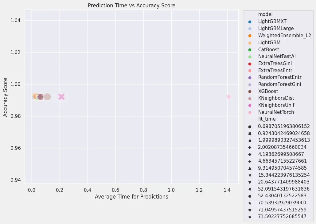
Model Training

predictor = TabularPredictor(label='LABEL', path=MODEL_PATH)
predictor.fit(train_data)

# AutoGluon training complete, total runtime = 315.97s ... Best model: "WeightedEnsemble_L2"

predictor.fit_summary()

	model	score_val	pred_time_val	fit_time
0	LightGBMXT	0.992	0.020418	15.344224
1	LightGBMLarge	0.992	0.022831	71.049574
2	WeightedEnsemble_L2	0.992	0.023695	71.592278
3	LightGBM	0.992	0.025427	20.643771
4	CatBoost	0.992	0.050176	70.539329
5	NeuralNetFastAI	0.992	0.050670	9.314951
6	ExtraTreesGini	0.992	0.057889	1.999989
7	ExtraTreesEntr	0.992	0.059487	2.002087
8	RandomForestEntr	0.992	0.059567	4.198627
9	RandomForestGini	0.992	0.062586	4.663457
10	XGBoost	0.992	0.064399	52.430401
11	KNeighborsDist	0.992	0.112409	0.698705
12	KNeighborsUnif	0.992	0.213056	0.924304
13	NeuralNetTorch	0.992	1.411860	52.091543

leaderboard=pd.DataFrame(predictor.leaderboard())

plt.figure(figsize=(8, 7))
sns.set(style='darkgrid')
sns.scatterplot(
    x='pred_time_val',
    y='score_val',
    data=leaderboard,
    s=300,
    alpha=0.5,
    hue='model',
    palette='tab20',
    style='fit_time'
)

plt.title('Prediction Time vs Accuracy Score')
plt.xlabel('Average Time for Predictions')
plt.ylabel('Accuracy Score')
plt.legend(bbox_to_anchor=(1.01,1.01))

plt.savefig('assets/Real_World_Model_to_Deployment_11.webp', bbox_inches='tight')

Model Evaluation

# load best model
predictor = TabularPredictor.load("model/")

data_test = TabularDataset('dataset/exoTest.csv')
# replacing label class [1,2] -> [0,1]
data_test = data_test.replace({'LABEL': {2:1, 1:0}})

X_test = data_test.drop(columns=['LABEL'] )
y_test = data_test['LABEL']

y_pred = predictor.predict(X_test)

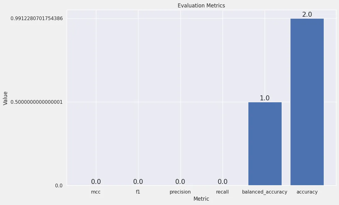
eval_metrics = predictor.evaluate_predictions(y_true=y_test, y_pred=y_pred, auxiliary_metrics=True)

# {
#     "accuracy": 0.9912280701754386,
#     "balanced_accuracy": 0.5000000000000001,
#     "mcc": 0.0,
#     "f1": 0.0,
#     "precision": 0.0,
#     "recall": 0.0
# }

array = np.array(list(eval_metrics.items()))
df = pd.DataFrame(array, columns = ['metric','value']).sort_values(by='value')

fig, ax =  plt.subplots(figsize = (10, 7))
ax.bar(df['metric'], df['value'])
for bar in ax.patches:
    ax.annotate(text = bar.get_height(),
                  xy = (bar.get_x() + bar.get_width() / 2, bar.get_height()),
                  ha='center', 
                  va='center',
                  size=15,
                  xytext=(0, 8),
                  textcoords='offset points')
plt.xlabel("Metric")
plt.ylabel("Value")
plt.title('Evaluation Metrics')
plt.ylim(bottom=0)

plt.savefig('assets/Real_World_Model_to_Deployment_12.webp', bbox_inches='tight')

Tabular Data Predictor on the re-balanced Dataset

As expected the results are badly affected by the inbalance of the dataset. Let's see how AutoGluon handles a preprocessed dataset.

Data Preprocessing

df_train = pd.read_csv('dataset/exoTrain.csv')
df_test = pd.read_csv('dataset/exoTest.csv')

df_train = df_train.replace({'LABEL': {2:1, 1:0}})
df_test = df_test.replace({'LABEL': {2:1, 1:0}})

X_train = df_train.drop(['LABEL'], axis=1)
y_train = df_train['LABEL']

X_test = df_test.drop(['LABEL'], axis=1)
y_test = df_test['LABEL']

# normalizing features
scaler = StandardScaler()
X_train_scaled = scaler.fit_transform(X_train)
X_test_scaled = scaler.fit_transform(X_test)

over_sampler = RandomOverSampler()
x_osample, y_osample = over_sampler.fit_resample(
    pd.DataFrame(X_train_scaled), y_train
)

df_merged_train = pd.concat([y_osample, x_osample], axis=1)
df_merged_train.head(5)

df_merged_test = pd.concat([y_test, pd.DataFrame(X_test_scaled)], axis=1)
df_merged_test.head(5)

df_merged_train.to_csv('dataset/exoTrainNorm.csv')
df_merged_test.to_csv('dataset/exoTestNorm.csv')

Model Training

data = TabularDataset('dataset/exoTrainNorm.csv')

print(len(data)*0.8)
# 8080.0

train_size = 8080
train_data = data.sample(n=train_size, random_state=SEED)
test_data = data.drop(train_data.index)
print(len(train_data), len(test_data))
# 8080 2020

predictor = TabularPredictor(label='LABEL', path=MODEL_PATH)
predictor.fit(train_data)

# AutoGluon training complete, total runtime = 412.18s ... Best model: "WeightedEnsemble_L2"

predictor.fit_summary()

	model	score_val	pred_time_val	fit_time
0	LightGBM	1.000000	0.029377	29.271464
1	LightGBMLarge	1.000000	0.037100	94.302897
2	CatBoost	1.000000	0.057690	79.490693
3	ExtraTreesGini	1.000000	0.063615	2.981032
4	ExtraTreesEntr	1.000000	0.064469	2.950440
5	RandomForestGini	1.000000	0.065542	6.167094
6	WeightedEnsemble_L2	1.000000	0.065813	3.676120
7	RandomForestEntr	1.000000	0.067343	6.783359
8	XGBoost	1.000000	0.099369	74.019001
9	NeuralNetTorch	1.000000	1.658319	26.595248
10	LightGBMXT	0.997525	0.027803	28.317720
11	KNeighborsDist	0.997525	0.367821	1.086449
12	KNeighborsUnif	0.997525	0.436408	0.956370
13	NeuralNetFastAI	0.986386	0.074977	20.446434

leaderboard=pd.DataFrame(predictor.leaderboard())

plt.figure(figsize=(8, 7))
sns.set(style='darkgrid')
sns.scatterplot(
    x='pred_time_val',
    y='score_val',
    data=leaderboard,
    s=300,
    alpha=0.5,
    hue='model',
    palette='tab20',
    style='fit_time'
)

plt.title('Prediction Time vs Accuracy Score')
plt.xlabel('Average Time for Predictions')
plt.ylabel('Accuracy Score')
plt.legend(bbox_to_anchor=(1.01,1.01))

plt.savefig('assets/Real_World_Model_to_Deployment_13.webp', bbox_inches='tight')

Model Evaluation

data_test = TabularDataset('dataset/exoTestNorm.csv')

X_test = data_test.drop(['LABEL'], axis=1)
y_test = data_test['LABEL']

# load best model
predictor = TabularPredictor.load("model/")

y_pred = predictor.predict(X_test)

eval_metrics = predictor.evaluate_predictions(y_true=y_test, y_pred=y_pred, auxiliary_metrics=True)

# {
#     "accuracy": 0.9912280701754386,
#     "balanced_accuracy": 0.5000000000000001,
#     "mcc": 0.0,
#     "f1": 0.0,
#     "precision": 0.0,
#     "recall": 0.0
# }

array = np.array(list(eval_metrics.items()))
df = pd.DataFrame(array, columns = ['metric','value']).sort_values(by='value')

fig, ax =  plt.subplots(figsize = (10, 7))
ax.bar(df['metric'], df['value'])
for bar in ax.patches:
    ax.annotate(text = bar.get_height(),
                  xy = (bar.get_x() + bar.get_width() / 2, bar.get_height()),
                  ha='center', 
                  va='center',
                  size=15,
                  xytext=(0, 8),
                  textcoords='offset points')
plt.xlabel("Metric")
plt.ylabel("Value")
plt.title('Evaluation Metrics')
plt.ylim(bottom=0)

plt.savefig('assets/Real_World_Model_to_Deployment_14.webp', bbox_inches='tight')

Multi Modal Predictor on the re-balanced Dataset

Data Preprocessing

data = TabularDataset('dataset/exoTrainNorm.csv')

train_data = data.sample(frac=0.8 , random_state=SEED)
test_data = data.drop(train_data.index)

Model Training

mm_predictor = MultiModalPredictor(label='LABEL', path=MODEL_PATH)

mm_predictor.fit(train_data)

Model Evaluation

mm_predictor = MultiModalPredictor.load('model/')

data_test = TabularDataset('dataset/exoTestNorm.csv')
X_test = data_test.drop(['LABEL'], axis=1)
y_test = data_test['LABEL']

model_scoring = mm_predictor.evaluate(data_test, metrics=['acc', 'f1'])
print(model_scoring)
# {'acc': 0.987719298245614, 'f1': 0.0}

data_test[2:8]
# check original dataframe to see labels - 3x1 and 3x0

		LABEL	0	1	2	3	4	5	6	7	...	3187	3188	3189	3190	3191	3192	3193	3194	3195	3196
2	2	1	0.026154	0.006299	0.018946	-0.005135	0.005965	-0.018322	-0.006160	-0.028589	...	-0.004433	-0.037509	-0.014466	-0.037624	-0.019497	-0.048315	-0.037617	-0.030012	-0.027607	-0.010661
3	3	1	-0.106614	-0.124118	-0.109998	-0.125241	-0.102100	-0.120553	-0.105169	-0.117242	...	0.006545	-0.022406	0.000427	-0.024211	-0.009926	-0.028069	-0.025272	-0.025595	-0.050906	-0.036046
4	4	1	-0.044110	-0.059779	-0.043223	-0.059295	-0.043759	-0.059998	-0.041655	-0.061203	...	-0.010283	-0.038573	-0.012238	-0.033583	-0.014463	-0.039068	-0.036145	-0.019389	-0.031042	-0.015661
5	5	0	-0.039830	-0.057677	-0.041331	-0.057802	-0.041504	-0.057055	-0.040597	-0.057336	...	-0.005900	-0.032540	-0.009752	-0.031495	-0.011695	-0.030716	-0.027901	-0.012041	-0.023759	-0.014598
6	6	0	-0.052925	-0.069757	-0.055066	-0.073462	-0.055658	-0.071925	-0.054675	-0.070939	...	-0.005554	-0.031578	-0.010334	-0.035450	-0.014312	-0.031091	-0.029233	-0.013697	-0.025068	-0.014998
7	7	0	-0.041764	-0.059533	-0.043542	-0.059569	-0.043982	-0.059702	-0.043419	-0.059123	...	-0.004048	-0.028919	-0.006828	-0.027940	-0.007229	-0.026500	-0.031011	-0.016102	-0.027207	-0.015900

# pick data without labels from test set
test_pred = X_test[2:8]

print(mm_predictor.class_labels)
mm_predictor.predict_proba(test_pred)

	0	1
2	0.990848	0.009152
3	0.873063	0.126937
4	0.989407	0.010593
5	0.993549	0.006451
6	0.983894	0.016106
7	0.993914	0.006086

Hmmmm so why doesn't this work?